Automobile Price Prediction

Project Team ID = PTID-CDS-JUL21-1171 (Members - Diana, Hema, Pavithra and Sophiya)

Project ID = PRCP-1001-RiceLeaf (Automobile Imports Price Prediction)

—— Preliminary → Identify The Business Case ——

This is an Automobile Imports Data Set which contains various characteristics of the cars including insurance risk rating and other price indicators. The target is to predict the price of the cars. Consequently, in order to avoid ‘the curse of dimensionality’, we’re gonna involve the top 10 of most influence features and will involve it to be a part of prediction journey (passing 10 selected features into X).
Because of main focus is to finding the most vigorous correlation that affecting price (target), the most opportune method to solve this case is by applying regression.

png
Image Credit

#Importing Important Libraries
import numpy as np
import pandas as pd
import matplotlib.pyplot as plt
import seaborn as sns
import warnings
warnings.filterwarnings("ignore")
from sklearn.impute import SimpleImputer
from sklearn.preprocessing import  LabelEncoder
from sklearn.feature_selection import SelectKBest
from sklearn.feature_selection import chi2
from sklearn.model_selection import train_test_split
from sklearn.preprocessing import StandardScaler
from sklearn.linear_model import LinearRegression
from sklearn.metrics import r2_score
from statsmodels.stats.outliers_influence import variance_inflation_factor
from sklearn.linear_model import Ridge
from sklearn.linear_model import Lasso
from sklearn.svm import SVR
from sklearn.model_selection import GridSearchCV
from sklearn.decomposition import PCA
import pickle


#Loading the dataset from .csv file, & rename each columns (as stated in the .txt file)
data =  pd.read_csv('auto_imports.csv', names=['symboling', 'normalized_losses', 'make', 'fuel_type', 'aspiration',
                                               'num_of_doors', 'body_style', 'drive_wheels', 'engine_location', 'wheel_base',
                                               'length', 'width', 'height', 'curb_weight', 'engine_type', 'num_of_cylinders',
                                               'engine_size', 'fuel_system', 'bore', 'stroke', 'compression_ratio', 'horsepower',
                                               'peak_rpm', 'city_mpg', 'highway_mpg', 'price'])
#show the data head
data.head().T

	0	1	2	3	4
symboling	3	3	1	2	2
normalized_losses	?	?	?	164	164
make	alfa-romero	alfa-romero	alfa-romero	audi	audi
fuel_type	gas	gas	gas	gas	gas
aspiration	std	std	std	std	std
num_of_doors	two	two	two	four	four
body_style	convertible	convertible	hatchback	sedan	sedan
drive_wheels	rwd	rwd	rwd	fwd	4wd
engine_location	front	front	front	front	front
wheel_base	88.6	88.6	94.5	99.8	99.4
length	168.8	168.8	171.2	176.6	176.6
width	64.1	64.1	65.5	66.2	66.4
height	48.8	48.8	52.4	54.3	54.3
curb_weight	2548	2548	2823	2337	2824
engine_type	dohc	dohc	ohcv	ohc	ohc
num_of_cylinders	four	four	six	four	five
engine_size	130	130	152	109	136
fuel_system	mpfi	mpfi	mpfi	mpfi	mpfi
bore	3.47	3.47	2.68	3.19	3.19
stroke	2.68	2.68	3.47	3.40	3.40
compression_ratio	9.0	9.0	9.0	10.0	8.0
horsepower	111	111	154	102	115
peak_rpm	5000	5000	5000	5500	5500
city_mpg	21	21	19	24	18
highway_mpg	27	27	26	30	22
price	13495	16500	16500	13950	17450

Predicated on the results above, the independent variable a.k.a X falls on the first row to 25 (in this case start from: 'symboling' - 'highway_mpg'). The last row is the dependent variable a.k.a Y (price).

——————— Dataset Information ———————

Description: This data set consists of three types of entities:

The specification of an auto in terms of various characteristics,
Its assigned insurance risk rating,
Its normalized losses in use as compared to other cars. The second rating corresponds to the degree to which the auto is more risky than its price indicates. Cars are initially assigned a risk factor symbol associated with its price. Then, if it is more risky (or less), this symbol is adjusted by moving it up (or down) the scale. Actuarians call this process “symboling”. A value of +3 indicates that the auto is risky, -3 that it is probably pretty safe.

The third factor is the relative average loss payment per insured vehicle year. This value is normalized for all autos within a particular size classification (two-door small, station wagons, sports/speciality, etc…), and represents the average loss per car per year.

Note: Several of the attributes in the database could be used as a “class” attribute.

symboling: -3, -2, -1, 0, 1, 2, 3.
normalized-losses: continuous from 65 to 256.
make: alfa-romero, audi, bmw, chevrolet, dodge, honda, isuzu, jaguar, mazda, mercedes-benz, mercury, mitsubishi, nissan, peugot, plymouth, porsche, renault, saab, subaru, toyota, volkswagen, volvo
fuel-type: diesel, gas.
aspiration: std, turbo.
num-of-doors: four, two.
body-style: hardtop, wagon, sedan, hatchback, convertible.
drive-wheels: 4wd, fwd, rwd.
engine-location: front, rear.
wheel-base: continuous from 86.6 120.9.
length: continuous from 141.1 to 208.1.
width: continuous from 60.3 to 72.3.
height: continuous from 47.8 to 59.8.
curb-weight: continuous from 1488 to 4066.
engine-type: dohc, dohcv, l, ohc, ohcf, ohcv, rotor.
num-of-cylinders: eight, five, four, six, three, twelve, two.
engine-size: continuous from 61 to 326.
fuel-system: 1bbl, 2bbl, 4bbl, idi, mfi, mpfi, spdi, spfi.
bore: continuous from 2.54 to 3.94.
stroke: continuous from 2.07 to 4.17.
compression-ratio: continuous from 7 to 23.
horsepower: continuous from 48 to 288.
peak-rpm: continuous from 4150 to 6600.
city-mpg: continuous from 13 to 49.
highway-mpg: continuous from 16 to 54.
price: continuous from 5118 to 45400.

print("____________________________________________")
print("            Info of The Dataset")
print("____________________________________________")
data.info() 

____________________________________________
            Info of The Dataset
____________________________________________
<class 'pandas.core.frame.DataFrame'>
RangeIndex: 201 entries, 0 to 200
Data columns (total 26 columns):
 #   Column             Non-Null Count  Dtype  
---  ------             --------------  -----  
 symboling          201 non-null    int64  
 normalized_losses  201 non-null    object 
 make               201 non-null    object 
 fuel_type          201 non-null    object 
 aspiration         201 non-null    object 
 num_of_doors       201 non-null    object 
 body_style         201 non-null    object 
 drive_wheels       201 non-null    object 
 engine_location    201 non-null    object 
 wheel_base         201 non-null    float64
length             201 non-null    float64
width              201 non-null    float64
height             201 non-null    float64
curb_weight        201 non-null    int64  
engine_type        201 non-null    object 
num_of_cylinders   201 non-null    object 
engine_size        201 non-null    int64  
fuel_system        201 non-null    object 
bore               201 non-null    object 
stroke             201 non-null    object 
compression_ratio  201 non-null    float64
horsepower         201 non-null    object 
peak_rpm           201 non-null    object 
city_mpg           201 non-null    int64  
highway_mpg        201 non-null    int64  
price              201 non-null    int64  
dtypes: float64(5), int64(6), object(15)
memory usage: 41.0+ KB

print("____________________________________________")
print("   Counting Missing Values of The Dataset")
print("____________________________________________")
data.isnull().sum()

____________________________________________
   Counting Missing Values of The Dataset
____________________________________________





symboling            0
normalized_losses    0
make                 0
fuel_type            0
aspiration           0
num_of_doors         0
body_style           0
drive_wheels         0
engine_location      0
wheel_base           0
length               0
width                0
height               0
curb_weight          0
engine_type          0
num_of_cylinders     0
engine_size          0
fuel_system          0
bore                 0
stroke               0
compression_ratio    0
horsepower           0
peak_rpm             0
city_mpg             0
highway_mpg          0
price                0
dtype: int64

Remarks - Several of columns have missing values, they are not being captured in the above as they are considered as strings (‘?’) and not missing values. To rectify it, superseding '?' with the avail of np.NaN

png
Image Credit

Replace ‘?’ with np.NaN, so the missing values can be filled.

data = data.replace('?', np.NaN)
data.head()

	symboling	normalized_losses	make	fuel_type	aspiration	num_of_doors	body_style	drive_wheels	engine_location	wheel_base	...	engine_size	fuel_system	bore	stroke	compression_ratio	horsepower	peak_rpm	city_mpg	highway_mpg	price
0	3	NaN	alfa-romero	gas	std	two	convertible	rwd	front	88.6	...	130	mpfi	3.47	2.68	9.0	111	5000	21	27	13495
1	3	NaN	alfa-romero	gas	std	two	convertible	rwd	front	88.6	...	130	mpfi	3.47	2.68	9.0	111	5000	21	27	16500
2	1	NaN	alfa-romero	gas	std	two	hatchback	rwd	front	94.5	...	152	mpfi	2.68	3.47	9.0	154	5000	19	26	16500
3	2	164	audi	gas	std	four	sedan	fwd	front	99.8	...	109	mpfi	3.19	3.40	10.0	102	5500	24	30	13950
4	2	164	audi	gas	std	four	sedan	4wd	front	99.4	...	136	mpfi	3.19	3.40	8.0	115	5500	18	22	17450

5 rows × 26 columns

Checking for the no. of missing values in each column

#displays features that have missing values in them
def missing_zero_values_table(data):
        zero_val = (data == 0.00).astype(int).sum(axis=0)
        mis_val = data.isnull().sum()
        mis_val_percent = 100 * data.isnull().sum() / len(data)
        mz_table = pd.concat([mis_val, mis_val_percent], axis=1)
        mz_table = mz_table.rename(
        columns = {0 : 'Sum of NaN', 1 : 'Total Values (%)'})
        mz_table['Data Type'] = data.dtypes
        mz_table = mz_table[
            mz_table.iloc[:,1] != 0].sort_values(
        'Total Values (%)', ascending=False).round(1)
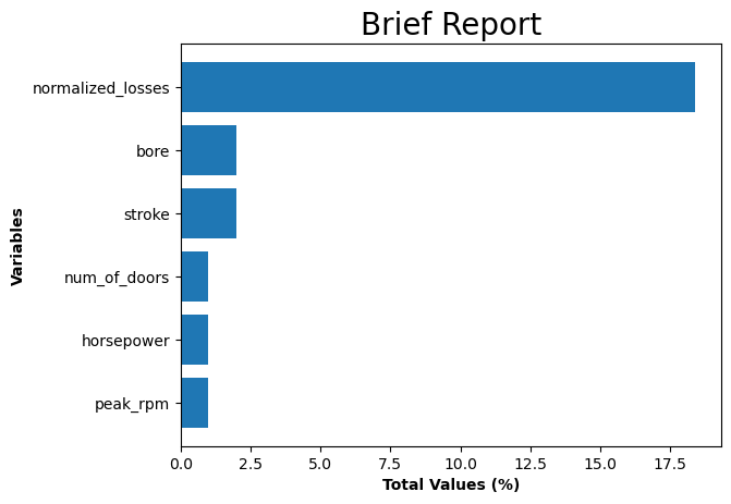
        print ("================= Brief Report =================\nData has " + str(data.shape[1]) + " columns and " + str(data.shape[0]) + " Rows.\n"      
            "There are " + str(mz_table.shape[0]) +
              " columns that have missing values as\nrepresented below:")
        return mz_table
missing_zero_values_table(data)

================= Brief Report =================
Data has 26 columns and 201 Rows.
There are 6 columns that have missing values as
represented below:

	Sum of NaN	Total Values (%)	Data Type
normalized_losses	37	18.4	object
bore	4	2.0	object
stroke	4	2.0	object
num_of_doors	2	1.0	object
horsepower	2	1.0	object
peak_rpm	2	1.0	object

#slice vars contains NaN values
slice_var = data[['normalized_losses', 'bore', 'stroke', 'num_of_doors', 'horsepower', 'peak_rpm']]
slice_var

#visualize it
plt.rcdefaults()
fig, ax = plt.subplots()

#columns contain missing values
var = ('normalized_losses', 'bore', 'stroke', 'num_of_doors', 'horsepower', 'peak_rpm')
y_pos = np.arange(len(var))
perc = 100 * slice_var.isnull().sum() / len(slice_var)

ax.barh(y_pos, perc, align = 'center')
ax.set_yticks(y_pos)
ax.set_yticklabels(slice_var)
ax.invert_yaxis()  # labels read top-to-bottom
ax.set_xlabel('Total Values (%)', fontweight='bold')
ax.set_ylabel('Variables', fontweight='bold')
ax.set_title('Brief Report', size = 20)
plt.savefig('[Fig 2.1] Brief Report.png', dpi = 300)
plt.show()

png

Interpretation:

There are 6 columns that have missing values.
Some of the columns are recorded as ‘object’ although they have values that are continuous.
Switching ‘object’ dtype to numeric for 5 columns (excluding ‘num_of_doors’) which is categorical variable.

data[['normalized_losses', 'bore', 'stroke', 'horsepower', 'peak_rpm']] = data[['normalized_losses', 'bore', 'stroke', 'horsepower', 'peak_rpm']].apply(pd.to_numeric)

# For the numerical values, replacing the missing values with mean of their respective columns

data['normalized_losses'].fillna(data['normalized_losses'].mean(), inplace = True)
data['bore'].fillna(data['bore'].mean(), inplace = True)
data['stroke'].fillna(data['stroke'].mean(), inplace = True)
data['horsepower'].fillna(data['horsepower'].mean(), inplace = True)
data['peak_rpm'].fillna(data['peak_rpm'].mean(), inplace = True)

# For the categorical value (num_of_doors), replacing the missing values with most frequently appearing values (mode)

imputer = SimpleImputer(strategy='most_frequent')

data.iloc[:,:] = imputer.fit_transform(data)

# re-execute previous functions (missing values)  
missing_zero_values_table(data)

================= Brief Report =================
Data has 26 columns and 201 Rows.
There are 0 columns that have missing values as
represented below:

	Sum of NaN	Total Values (%)	Data Type

Missing Values has been completely handle.

data.describe().T

	count	mean	std	min	25%	50%	75%	max
symboling	201.0	0.840796	1.254802	-2.00	0.00	1.00000	2.00	3.00
normalized_losses	201.0	122.000000	31.996250	65.00	101.00	122.00000	137.00	256.00
wheel_base	201.0	98.797015	6.066366	86.60	94.50	97.00000	102.40	120.90
length	201.0	174.200995	12.322175	141.10	166.80	173.20000	183.50	208.10
width	201.0	65.889055	2.101471	60.30	64.10	65.50000	66.60	72.00
height	201.0	53.766667	2.447822	47.80	52.00	54.10000	55.50	59.80
curb_weight	201.0	2555.666667	517.296727	1488.00	2169.00	2414.00000	2926.00	4066.00
engine_size	201.0	126.875622	41.546834	61.00	98.00	120.00000	141.00	326.00
bore	201.0	3.330711	0.268072	2.54	3.15	3.31000	3.58	3.94
stroke	201.0	3.256904	0.316048	2.07	3.11	3.29000	3.41	4.17
compression_ratio	201.0	10.164279	4.004965	7.00	8.60	9.00000	9.40	23.00
horsepower	201.0	103.396985	37.365602	48.00	70.00	95.00000	116.00	262.00
peak_rpm	201.0	5117.587940	478.113178	4150.00	4800.00	5117.58794	5500.00	6600.00
city_mpg	201.0	25.179104	6.423220	13.00	19.00	24.00000	30.00	49.00
highway_mpg	201.0	30.686567	6.815150	16.00	25.00	30.00000	34.00	54.00
price	201.0	13207.129353	7947.066342	5118.00	7775.00	10295.00000	16500.00	45400.00

Encoding the categorical variables for model building using LabelEncoder

label = LabelEncoder()
data1 = data.apply(label.fit_transform)
data1.head()

	symboling	normalized_losses	make	fuel_type	num_of_doors	body_style	drive_wheels	wheel_base	...	engine_size	fuel_system	bore	stroke	compression_ratio	horsepower	peak_rpm	city_mpg	highway_mpg	price
0	5	28	0	1	1	0	2	2	...	18	5	24	4	13	31	10	8	10	117
1	5	28	0	1	1	0	2	2	...	18	5	24	4	13	31	10	8	10	136
2	3	28	0	1	1	2	2	10	...	28	5	1	28	13	46	10	6	9	136
3	4	42	1	1	0	3	1	29	...	11	5	13	25	22	27	17	11	13	122
4	4	42	1	1	0	3	0	28	...	22	5	13	25	5	34	17	5	5	147

5 rows × 26 columns

Cross Checking if the label encoder has encoded all the values properly

#head of dataset (data types 'object' only)

data.select_dtypes(include = 'object').head()

	make	fuel_type	aspiration	num_of_doors	body_style	drive_wheels	engine_location	engine_type	num_of_cylinders	fuel_system
0	alfa-romero	gas	std	two	convertible	rwd	front	dohc	four	mpfi
1	alfa-romero	gas	std	two	convertible	rwd	front	dohc	four	mpfi
2	alfa-romero	gas	std	two	hatchback	rwd	front	ohcv	six	mpfi
3	audi	gas	std	four	sedan	fwd	front	ohc	four	mpfi
4	audi	gas	std	four	sedan	4wd	front	ohc	five	mpfi

print('-------------------------------------------------------- 1. [make] ----------------------------------------------------------')
print('Categorical Values: ',data.make.unique())
print('Numerical Values: ',data1.make.unique(), '\n')
print('----------------------------------------------------- 2. [fuel_type] --------------------------------------------------------')
print('Categorical Values: ',data.fuel_type.unique())
print('Numerical Values: ',data1.fuel_type.unique(), '\n')
print('----------------------------------------------------- 3. [aspiration] --------------------------------------------------------')
print('Categorical Values: ',data.aspiration.unique())
print('Numerical Values: ',data1.aspiration.unique(), '\n')
print('---------------------------------------------------- 4. [num_of_doors] -------------------------------------------------------')
print('Categorical Values: ',data.num_of_doors.unique())
print('Numerical Values: ',data1.num_of_doors.unique(), '\n')
print('----------------------------------------------------- 5. [body_style] --------------------------------------------------------')
print('Categorical Values: ',data.body_style.unique())
print('Numerical Values: ',data1.body_style.unique(), '\n')
print('---------------------------------------------------- 6. [drive_wheels] -------------------------------------------------------')
print('Categorical Values: ',data.drive_wheels.unique())
print('Numerical Values: ',data1.drive_wheels.unique(), '\n')
print('--------------------------------------------------- 7. [engine_location] ------------------------------------------------------')
print('Categorical Values: ',data.engine_location.unique())
print('Numerical Values: ',data1.engine_location.unique(),'\n')
print('----------------------------------------------------- 8. [engine_type] --------------------------------------------------------')
print('Categorical Values: ',data.engine_type.unique())
print('Numerical Values: ',data1.engine_type.unique(),'\n')
print('-------------------------------------------------- 9. [num_of_cylinders] -----------------------------------------------------')
print('Categorical Values: ',data.num_of_cylinders.unique())
print('Numerical Values: ',data1.num_of_cylinders.unique(),'\n')
print('---------------------------------------------------- 10. [fuel_system] -------------------------------------------------------')
print('Categorical Values: ',data.fuel_system.unique())
print('Numerical Values: ',data1.fuel_system.unique(), '\n')

-------------------------------------------------------- 1. [make] ----------------------------------------------------------
Categorical Values:  ['alfa-romero' 'audi' 'bmw' 'chevrolet' 'dodge' 'honda' 'isuzu' 'jaguar'
 'mazda' 'mercedes-benz' 'mercury' 'mitsubishi' 'nissan' 'peugot'
 'plymouth' 'porsche' 'renault' 'saab' 'subaru' 'toyota' 'volkswagen'
 'volvo']
Numerical Values:  [ 0  1  2  3  4  5  6  7  8  9 10 11 12 13 14 15 16 17 18 19 20 21] 

----------------------------------------------------- 2. [fuel_type] --------------------------------------------------------
Categorical Values:  ['gas' 'diesel']
Numerical Values:  [1 0] 

----------------------------------------------------- 3. [aspiration] --------------------------------------------------------
Categorical Values:  ['std' 'turbo']
Numerical Values:  [0 1] 

---------------------------------------------------- 4. [num_of_doors] -------------------------------------------------------
Categorical Values:  ['two' 'four']
Numerical Values:  [1 0] 

----------------------------------------------------- 5. [body_style] --------------------------------------------------------
Categorical Values:  ['convertible' 'hatchback' 'sedan' 'wagon' 'hardtop']
Numerical Values:  [0 2 3 4 1] 

---------------------------------------------------- 6. [drive_wheels] -------------------------------------------------------
Categorical Values:  ['rwd' 'fwd' '4wd']
Numerical Values:  [2 1 0] 

--------------------------------------------------- 7. [engine_location] ------------------------------------------------------
Categorical Values:  ['front' 'rear']
Numerical Values:  [0 1] 

----------------------------------------------------- 8. [engine_type] --------------------------------------------------------
Categorical Values:  ['dohc' 'ohcv' 'ohc' 'l' 'rotor' 'ohcf']
Numerical Values:  [0 4 2 1 5 3] 

-------------------------------------------------- 9. [num_of_cylinders] -----------------------------------------------------
Categorical Values:  ['four' 'six' 'five' 'three' 'twelve' 'two' 'eight']
Numerical Values:  [2 3 1 4 5 6 0] 

---------------------------------------------------- 10. [fuel_system] -------------------------------------------------------
Categorical Values:  ['mpfi' '2bbl' 'mfi' '1bbl' 'spfi' '4bbl' 'idi' 'spdi']
Numerical Values:  [5 1 4 0 7 2 3 6] 

# splitting the data into X and Y so we can do feature selection

x  = data1.drop('price', axis=1)
y = data1['price']
print(x.head())
y.head()

   symboling  normalized_losses  make  fuel_type  aspiration  num_of_doors  \
        5                 28     0          1           0             1   
        5                 28     0          1           0             1   
        3                 28     0          1           0             1   
        4                 42     1          1           0             0   
        4                 42     1          1           0             0   

   body_style  drive_wheels  engine_location  wheel_base  ...  \
         0             2                0           2  ...   
         0             2                0           2  ...   
         2             2                0          10  ...   
         3             1                0          29  ...   
         3             0                0          28  ...   

   num_of_cylinders  engine_size  fuel_system  bore  stroke  \
               2           18            5    24       4   
               2           18            5    24       4   
               3           28            5     1      28   
               2           11            5    13      25   
               1           22            5    13      25   

   compression_ratio  horsepower  peak_rpm  city_mpg  highway_mpg  
               13          31        10         8           10  
               13          31        10         8           10  
               13          46        10         6            9  
               22          27        17        11           13  
                5          34        17         5            5  

[5 rows x 25 columns]





  117
  136
  136
  122
  147
Name: price, dtype: int64

Remarks - Data is now cleaned (missing values are filled and all the categorical variables are, and ready for analysis.)
Disclaimer - One hot encoder etc. were not used although there is a risk of the encoded values being ranked based on the encoded values and may be considered to be more important than the others in the regression analysis.

#saving cleaned data to .csv files
data1.to_csv('auto_imports [cleaned].csv', index=False)

At this time we have chosen not to add more variables (over 50) into the mix with the other forms of encoding as we have performed feature selection analysis to reduce the dimensions for modeling. In the event any of the categorical variables are selected as an important feature by the feature selection technique then we would use other forms of encoding and add the new encoded variables to the predictor data set to do the modeling.

# FEATURE SELECTION TECHNIQUE
#apply SelectKBest class to extract top 10 best features
bestfeatures = SelectKBest(score_func=chi2, k=10)
fit = bestfeatures.fit(x,y)
dfscores = pd.DataFrame(fit.scores_)
dfcolumns = pd.DataFrame(x.columns)

#concat two dataframes for better visualization
featurescores = pd.concat([dfcolumns,dfscores], axis=1)
featurescores.columns = ['Specs', 'Score'] #naming the data
print(featurescores.nlargest(10, 'Score'))

                Specs        Score
      curb_weight  5691.994803
           length  2319.534038
       horsepower  1865.324072
        wheel_base  1657.488294
           height  1435.530316
      engine_size  1367.586605
 normalized_losses  1285.230854
            width  1277.660011
             bore  1124.427128
           stroke   790.046992

The top 10 features are now used to build the models for comparison

Modifying The Dataset by Including These 10 Selected Features

X = x[['curb_weight', 'length', 'horsepower','wheel_base','height','engine_size','normalized_losses','width','bore','stroke']].copy()
X.head()

	curb_weight	length	horsepower	wheel_base	height	engine_size	normalized_losses	width	bore	stroke
0	92	22	31	2	1	18	28	8	24	4
1	92	22	31	2	1	18	28	8	24	4
2	115	29	46	10	13	28	28	16	1	28
3	66	44	27	29	25	11	42	21	13	25
4	116	44	34	28	25	22	42	23	13	25

png
Image Credit

# Checking for the skewness and kurtosis for 10 selected features and target

print("Skewness of curb_weight: %f" %X['curb_weight'].skew())
print("Kurtosis of curb_weight: %f" %X['curb_weight'].kurt())
print("Skewness of length: %f" %X['length'].skew())
print("Kurtosis of length: %f" %X['length'].kurt())
print("Skewness of horsepower: %f" %X['horsepower'].skew())
print("Kurtosis of horsepower: %f" %X['horsepower'].kurt())
print("Skewness of wheel_base: %f" %X['wheel_base'].skew())
print("Kurtosis of wheel_base: %f" %X['wheel_base'].kurt())
print("Skewness of height: %f" %X['height'].skew())
print("Kurtosis of height: %f" %X['height'].kurt())
print("Skewness of engine_size: %f" %X['engine_size'].skew())
print("Kurtosis of engine_size %f" %X['engine_size'].kurt())
print("Skewness of normalized_losses: %f" %X['normalized_losses'].skew())
print("Kurtosis of normalized_losses: %f" %X['normalized_losses'].kurt())
print("Skewness of width: %f" %X['width'].skew())
print("Kurtosis of width: %f" %X['width'].kurt())
print("Skewness of bore: %f" %X['bore'].skew())
print("Kurtosis of bore: %f" %X['bore'].kurt())
print("Skewness of stroke: %f" %X['stroke'].skew())
print("Kurtosis of stroke: %f" %X['stroke'].kurt())
print("Skewness of Price: %f" %data1['price'].skew())
print("Kurtosis of Price: %f" %data1['price'].kurt())

Skewness of curb_weight: 0.093721
Kurtosis of curb_weight: -1.147269
Skewness of length: 0.019671
Kurtosis of length: -1.176374
Skewness of horsepower: 0.430146
Kurtosis of horsepower: -0.886195
Skewness of wheel_base: 0.449951
Kurtosis of wheel_base: -0.955813
Skewness of height: 0.097420
Kurtosis of height: -1.143859
Skewness of engine_size: 0.623072
Kurtosis of engine_size -0.766610
Skewness of normalized_losses: -0.176570
Kurtosis of normalized_losses: -0.842252
Skewness of width: 0.381469
Kurtosis of width: -0.888932
Skewness of bore: 0.131851
Kurtosis of bore: -1.187268
Skewness of stroke: -0.368742
Kurtosis of stroke: -0.759355
Skewness of Price: 0.066486
Kurtosis of Price: -1.204690

Reference: Skewness between -0.5 and 0.5: data fairly symmetrical. Skewness between -1 and – 0.5 or between 0.5 and 1: data moderately skewed. Skewness < -1 or > than 1: the data are highly skewed. Kurtosis between -2 and +2 are considered acceptable.

Teams Remarks: The Skewness and Kurtosis for all the predictor and target variables falls within the acceptable range.

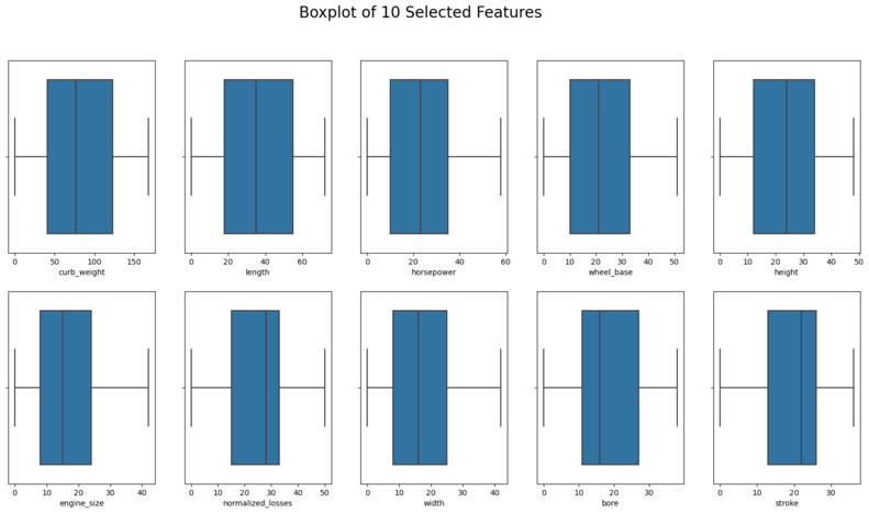
#Boxplot analysis

figure, ax = plt.subplots(2,5, figsize=(20,10))


plt.suptitle('Boxplot of 10 Selected Features', size = 20)
sns.boxplot(data1['curb_weight'],ax=ax[0,0])
sns.boxplot(data1['length'], ax=ax[0,1])
sns.boxplot(data1['horsepower'], ax=ax[0,2])
sns.boxplot(data1['wheel_base'], ax=ax[0,3])
sns.boxplot(data1['height'], ax=ax[0,4])
sns.boxplot(data1['engine_size'], ax=ax[1,0])
sns.boxplot(data1['normalized_losses'], ax=ax[1,1])
sns.boxplot(data1['width'], ax=ax[1,2])
sns.boxplot(data1['bore'], ax=ax[1,3])
sns.boxplot(data1['stroke'], ax=ax[1,4])
plt.savefig('[Fig 3.1] Boxplot of 10 Selected Features.png', dpi = 300)
plt.show()

png

figure, ax = plt.subplots(2,5, figsize=(20,10))

#See the distribution of the data

plt.suptitle('Distribution of 10 Selected Features', size = 20)
sns.distplot(data1['curb_weight'],ax=ax[0,0])
sns.distplot(data1['length'], ax=ax[0,1])
sns.distplot(data1['horsepower'], ax=ax[0,2])
sns.distplot(data1['wheel_base'], ax=ax[0,3])
sns.distplot(data1['height'], ax=ax[0,4])
sns.distplot(data1['engine_size'], ax=ax[1,0])
sns.distplot(data1['normalized_losses'], ax=ax[1,1])
sns.distplot(data1['width'], ax=ax[1,2])
sns.distplot(data1['bore'], ax=ax[1,3])
sns.distplot(data1['stroke'], ax=ax[1,4])
plt.savefig('[Fig 3.2] Distribution of 10 Selected Features.png', dpi = 300)
plt.show()

png

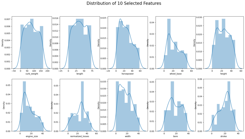
Interpretation: Boxplot and distribution plots look fine.

#combining the x (features) and y (target) to show the heatmap and pairplot analysis

xydata = data1[['curb_weight', 'length', 'horsepower','wheel_base','height','engine_size','normalized_losses','width','bore','stroke', 'price']].copy()

xydata.head()

	curb_weight	length	horsepower	wheel_base	height	engine_size	normalized_losses	width	bore	stroke	price
0	92	22	31	2	1	18	28	8	24	4	117
1	92	22	31	2	1	18	28	8	24	4	136
2	115	29	46	10	13	28	28	16	1	28	136
3	66	44	27	29	25	11	42	21	13	25	122
4	116	44	34	28	25	22	42	23	13	25	147

#Heatmap to shows the correlation

plt.figure(figsize=(20,15))
sns.heatmap(xydata.corr(),cmap='nipy_spectral',annot=True)
plt.title('Heatmap of 10 Selected Features and Target',
         fontsize=25)
plt.savefig('[Fig 3.3] Heatmap of 10 Selected Features and Target.png', dpi = 300)
plt.show()

png

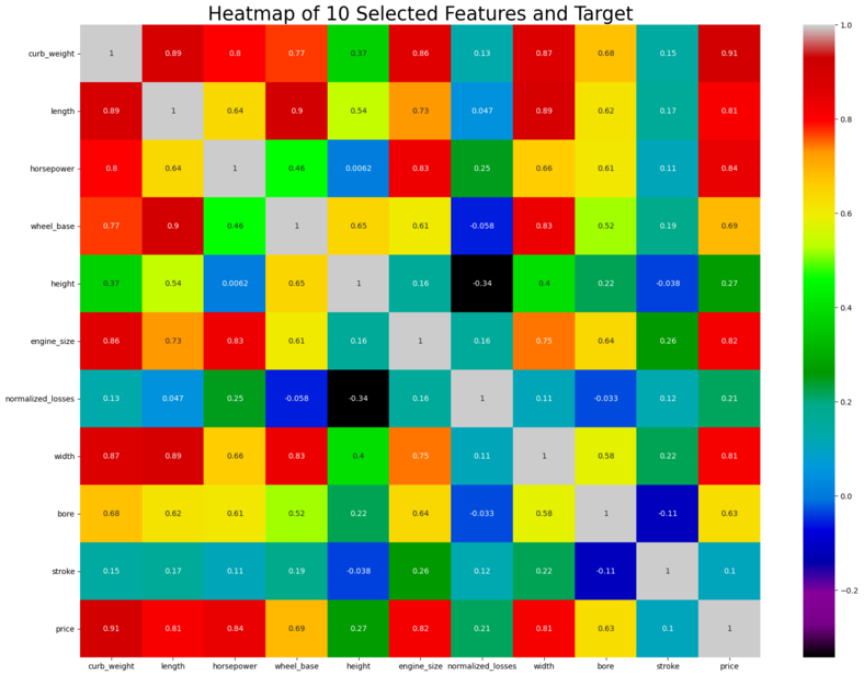
Teams Remarks: There seems to be significant amount of positive correlation between some of the predictor variables. Multicollinearity occurs when independent variables in a regression model are correlated. This correlation is a problem because independent variables should be independent. If the degree of correlation between variables is high enough, it can cause problems when we fit the model and interpret the results.

curb_weight is correlated to length, horsepower, wheelbase, enginesize, width and bore. Length is correlated to wheelbase and width. horsepower is correlated to engine size. Wheelbase is correlated to horsepower and width

Multicollinearity analysis is to be done in detail. See below

# Pairplot analysis
sns.pairplot(xydata)
plt.savefig('[Fig 3.4] Pairplot of 10 Selected Features and Target.png', dpi = 300)
plt.show()

png

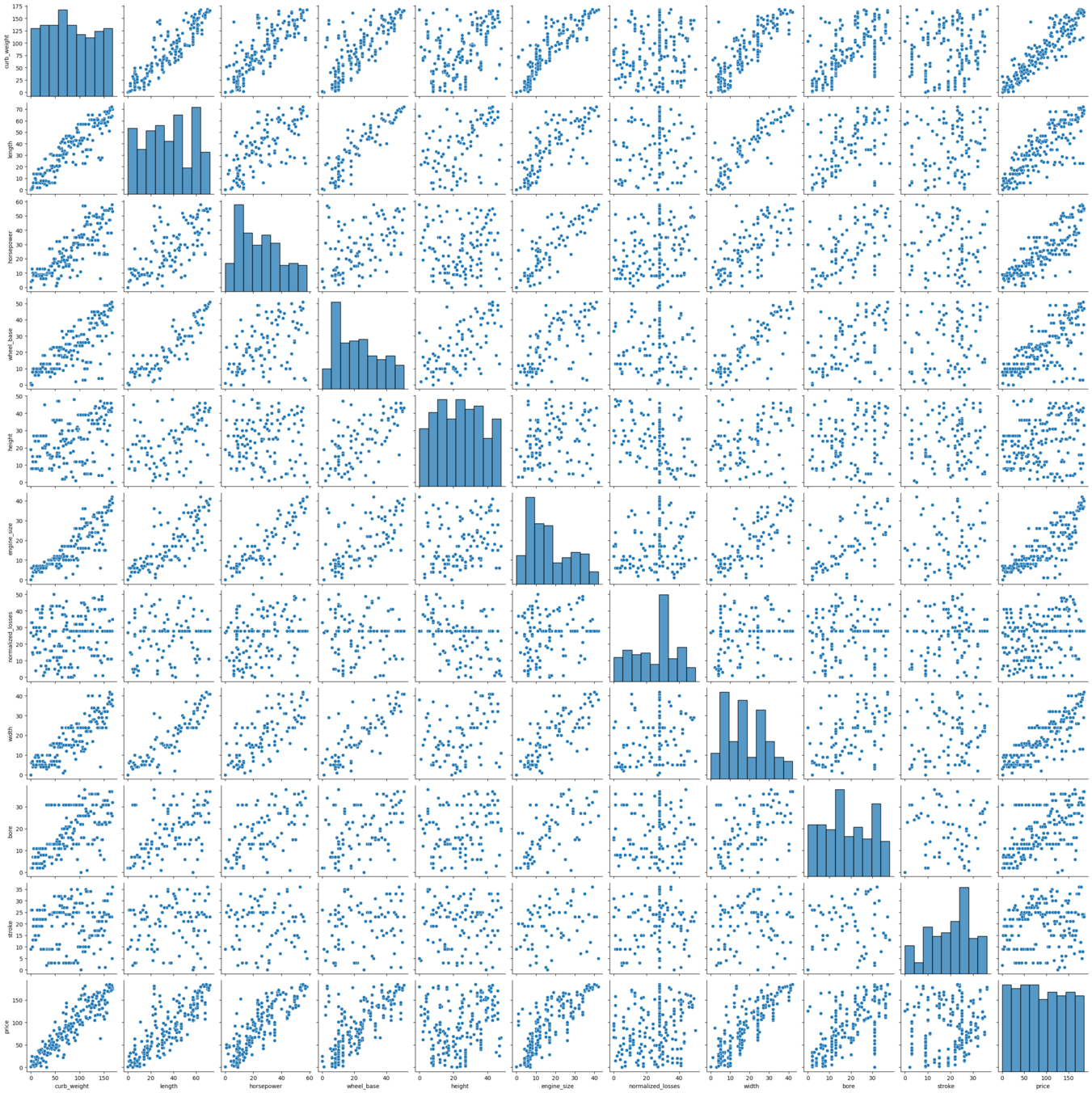
Remarks: As is evident from the pair plots, the target variable is showing a nice linear fit with some of the predictor variables. So, linear regression would provide felicitous model to the dataset.

Also there seems to be a linear relationship between some of the predictor variables, which is natural as the curb weight is dependent on the length, width and engine_size of the cars. This multicollinearity problem will be resolved by PCA analysis.

Residual plots to see if there are any patterns that could cause errors in the regression models.

figure, ax = plt.subplots(2,5, figsize=(20,10))

#See the Residual plots of the data

plt.suptitle('Residual Plot of 10 Selected Features Against Target', size = 20)
sns.residplot(data1['curb_weight'],data1['price'],ax=ax[0,0])
sns.residplot(data1['length'], data1['price'], ax=ax[0,1])
sns.residplot(data1['horsepower'], data1['price'], ax=ax[0,2])
sns.residplot(data1['wheel_base'], data1['price'], ax=ax[0,3])
sns.residplot(data1['height'], data1['price'], ax=ax[0,4])
sns.residplot(data1['engine_size'], data1['price'], ax=ax[1,0])
sns.residplot(data1['normalized_losses'], data1['price'], ax=ax[1,1])
sns.residplot(data1['width'], data1['price'], ax=ax[1,2])
sns.residplot(data1['bore'], data1['price'], ax=ax[1,3])
sns.residplot(data1['stroke'], data1['price'], ax=ax[1,4])
plt.savefig('[Fig 3.5] Residual Plot of 10 Selected Features Against Target.png', dpi = 300)
plt.show()

png

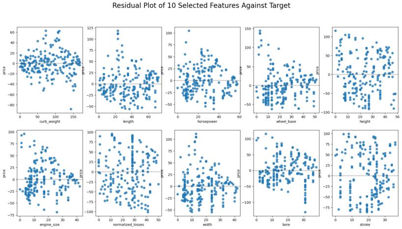
Remarks: No significant patterns in the residual plots

png
Image Credit

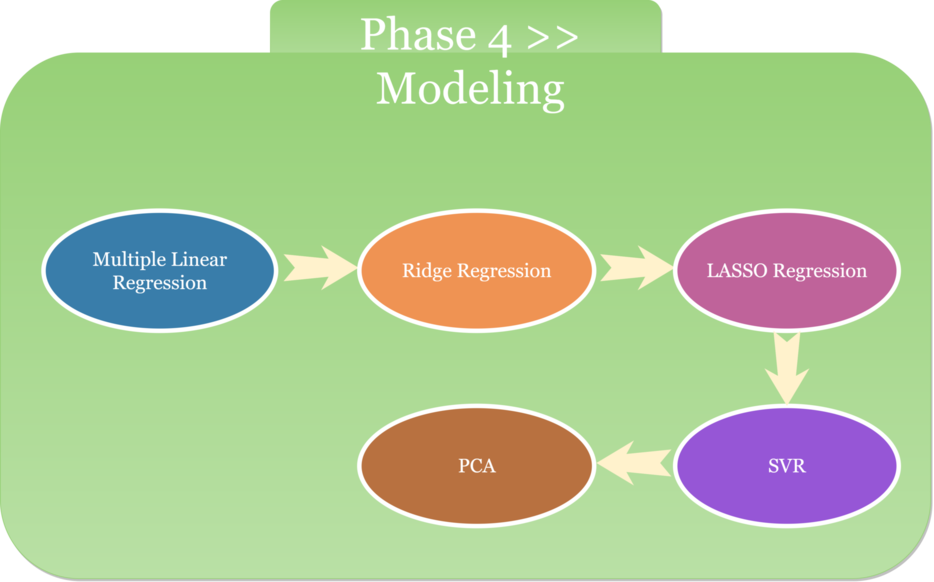
We vigorously believe when it comes to ML algorithm, "One Size Does Not Fit All". The same things additionally occur when it comes to modeling. To resolve the issue, several regression models will be utilized for the comparative analysis and the best model (shown by r2 score) will be chosen for this project.
Model 1: Multiple Linear Regression
Model 2: Ridge Regression
Model 3: Lasso Regression
Model 4: Support Vector Regression
Model 5: Principal Component Analysis (PCA)

Splitting the dataset into train and test data sets for validation

X_train, X_test, y_train, y_test = train_test_split(X, y, test_size=0.33, random_state=42)
X_train.shape, X_test.shape, y_train.shape, y_test.shape

((134, 10), (67, 10), (134,), (67,))

#feature scaling
sc = StandardScaler()
X_train_fc = sc.fit_transform(X_train)
X_test_fc = sc.transform(X_test)

Model 1: Multiple Linear Regression

# building the linear regression model
lm=LinearRegression()

# fitting the model with the standardized data
lm.fit(X_train_fc,y_train)

LinearRegression()

# predicting with the linear model
y_pred=lm.predict(X_test_fc)
Linear_Regr_score = r2_score(y_test,y_pred)
Linear_Regr_score

0.8675330801508967

Pickling The Model (Save and Load The Model)

with open('[4.1.1] Multiple_LR', 'wb') as f:
    pickle.dump(lm, f)
with open('[4.1.1] Multiple_LR', 'rb') as f:
    model_mlr = pickle.load(f)
#testing the pickled model. reason: to make sure the pickle output showing the same as the current model (y_pred)
model_mlr.predict(X_test_fc)

array([ 39.27873438, 172.39008554,  23.79690875,  38.81598645,
       118.02560264,  24.27532209, 166.90033166,  78.36283435,
       163.91513232, 182.72922042, 149.71410486,  56.22400104,
       108.4322148 ,  77.68539223, 113.30317396,  49.2278126 ,
        82.63551223,  35.51762066,  74.26413099, 178.80950224,
       125.98704081, 179.6828716 ,  19.49939044,  30.30081594,
       154.13705213,  74.45561159,  98.72363617, 159.9344475 ,
       128.14370608, 148.09795606, 102.11328533,  17.0646285 ,
       115.37359601,  38.42050953,  40.86989298, 138.82835563,
        28.40460768,  53.41603648, 106.81471585,  65.3142471 ,
       126.20111039, 140.32820502,  62.90172307,  34.66597309,
       128.76048409, 131.86746884,  12.84386201,  17.43809555,
        81.15455802,  23.63177825, 163.92478736, 162.83679969,
       105.50518899, 103.04129662,  34.36741024,  31.95051374,
        69.67767341, 150.74724269,  81.05866593,  74.96955417,
        74.50898045,  73.35205522,  12.8711576 , 127.07701526,
        28.46784132,  49.29817804,  60.93400171])

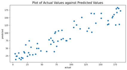
#Plot of Actual Values against Predicted Values
plt.figure(figsize=(10,5))
plt.scatter(y_test,y_pred)
plt.xlabel("actual")
plt.ylabel("predicted")
plt.title('Plot of Actual Values against Predicted Values',size = 15)
plt.savefig('[Fig 4.1] MultiLinReg Actual Against Target.png', dpi = 300)
plt.show()

png

Checking to see if the score can be improved if multicollinearity issue is resolved.
The potential solutions for resolving multicollinearity issues among the predictor variables are:

Remove some of the highly correlated independent variables.
Linearly combine the independent variables, such as adding them together.
Perform an analysis designed for highly correlated variables, such as principal components analysis or partial least squares regression.
Lasso and Ridge regression are advanced forms of regression analysis that can handle multicollinearity.

Improving the model - Iteration 1

N.B: Using the first solution from the above and reducing some of the highly correlated independent variables.

Part 1 - According to heatmap visualization, removing those predictor variables that show low correlation with target variables (stroke 0.1, normalized losses 0.21 and height 0.27), new X data set was made.

X_new = x[['curb_weight', 'length', 'horsepower','wheel_base','engine_size','width','bore']].copy()
X_new.head()

	curb_weight	length	horsepower	wheel_base	engine_size	width	bore
0	92	22	31	2	18	8	24
1	92	22	31	2	18	8	24
2	115	29	46	10	28	16	1
3	66	44	27	29	11	21	13
4	116	44	34	28	22	23	13

#creating train and test data set
X_trn_new, X_tst_new, y_trn_new, y_tst_new = train_test_split(X_new, y, test_size=0.33, random_state=42)
X_trn_new.shape, X_tst_new.shape, y_trn_new.shape, y_tst_new.shape

# scaling the features
X_trn_new_fc = sc.fit_transform(X_trn_new)
X_tst_new_fc = sc.transform(X_tst_new)

#fitting the model
lm.fit(X_trn_new_fc,y_trn_new)

# predicting using the test dataset
y_pred_new = lm.predict(X_tst_new_fc)

#checking the r2score using the new dataset
r2_score(y_tst_new,y_pred_new)

0.8780153528258652

Pickling The Model (Save and Load The Model)

with open('[4.1.2] Multiple_LR (Reduce Features According to Heatmap)', 'wb') as f:
    pickle.dump(lm, f)
with open('[4.1.2] Multiple_LR (Reduce Features According to Heatmap)', 'rb') as f:
    model_mlr = pickle.load(f)
#testing the pickled model. reason: to make sure the pickle output showing the same as the current model (y_pred_new)
model_mlr.predict(X_tst_new_fc)

array([ 29.86454227, 171.6891113 ,  22.1486513 ,  42.82401536,
       112.11902126,  22.46252551, 167.60650606,  89.02408535,
       155.05415392, 182.05624926, 158.03624213,  62.34155084,
       104.18416228,  70.59730038, 113.5235974 ,  47.40173449,
        79.14340238,  39.43691677,  71.86982329, 177.99817272,
       126.81306507, 180.64632423,  27.08085981,  27.93783444,
       162.6240674 ,  72.43507378,  98.88925128, 168.07217211,
       129.0711308 , 144.28285008,  87.10858806,  19.29036592,
       113.36858606,  31.34724299,  48.3701066 , 131.16942701,
        32.76502916,  51.32203631, 102.49061298,  60.10549721,
       129.04760861, 143.19642466,  71.99640675,  28.67220626,
       124.26122654, 134.65816999,  10.35967481,  23.94054364,
        84.37075626,  20.0346044 , 156.667191  , 153.92512106,
       104.10954835, 105.78034077,  26.97865696,  24.57304582,
        69.29689364, 150.09972471,  91.84666751,  77.43007886,
        84.37297962,  75.73652957,  15.69246978, 115.5654485 ,
        39.05066241,  41.80314572,  57.37789719])

Remarks: Score seemed to have improved slightly but no significant improvement
Improving the model - Iteration 2
N.B: only including the first four predictor variables that have the highest VIF values

VIF is used as a measure to check the strength of multicollinearity.

# VIF dataframe
vif_data = pd.DataFrame()
vif_data["feature"] = X_new.columns
  
# calculating VIF for each feature
vif_data["VIF"] = [variance_inflation_factor(X_new.values, i)
                          for i in range(len(X_new.columns))]
  
print(vif_data)

       feature        VIF
curb_weight  40.060008
     length  46.569846
 horsepower  14.498971
 wheel_base  23.567041
engine_size  17.044365
      width  22.841830
       bore   7.273853

References: VIF’s start at 1 and have no upper limit. A value of 1 indicates that there is no correlation between this independent variable and any others. VIF’s between 1 and 5 suggest that there is a moderate correlation, but it is not severe enough to warrant corrective measures. VIF’s > 5 represent critical levels of multicollinearity where the coefficients are poorly estimated, and the p-values are questionable.

Interpretation: based on the above length seems to have the highest VIF as it is heavily correlated to the curb_weight (which makes sense).

Decision: eliminating the features, creating a new data set, re-executing the model, checking the r2score below.

# creating a leaner data set
X_lean = x[['curb_weight', 'horsepower','wheel_base', 'engine_size', 'width', 'bore']].copy()

# training and splitting the data set
X_trn_lean, X_tst_lean, y_trn_lean, y_tst_lean = train_test_split(X_lean, y, test_size=0.33, random_state=42)
print(X_trn_lean.shape, X_tst_lean.shape, y_trn_lean.shape, y_tst_lean.shape)

# scaling the data set
X_trn_lean_fc = sc.fit_transform(X_trn_lean)
X_tst_lean_fc = sc.transform(X_tst_lean)

#fitting the model
lm.fit(X_trn_lean_fc,y_trn_lean)

# predicting the test data
y_pred_lean = lm.predict(X_tst_lean_fc)

# checking the R2 score
linear_FinalRegr_score = r2_score(y_tst_lean,y_pred_lean)
linear_FinalRegr_score

(134, 6) (67, 6) (134,) (67,)

0.8798334755333546

r2score has improved slightly

Pickling The Model (Save and Load The Model)

with open('[4.1.3] Multiple_LR (Applied VIF)', 'wb') as f:
    pickle.dump(lm, f)
with open('[4.1.3] Multiple_LR (Applied VIF)', 'rb') as f:
    model_mlr = pickle.load(f)
#testing the pickled model. reason: to make sure the pickle output showing the same as the current model (y_pred_lean)
model_mlr.predict(X_tst_lean_fc)

array([ 30.27343398, 170.47430895,  22.73895155,  43.36469706,
       109.23075799,  23.32399729, 167.69098889,  89.50820236,
       154.98421213, 182.45706477, 159.56262655,  62.73896071,
       103.07445564,  69.30465751, 112.65093414,  47.39745066,
        77.26159754,  39.80364378,  71.08518415, 178.75513972,
       126.99124146, 181.54374011,  28.54858269,  27.66585924,
       164.05783674,  70.67878124,  98.51475024, 168.88227382,
       129.36527698, 142.05415334,  85.75650386,  20.82564877,
       114.89414291,  32.96710779,  46.94735796, 132.15850514,
        34.18564324,  50.85908724, 101.293929  ,  61.53487905,
       129.33993144, 143.76753303,  69.19369441,  29.85259497,
       127.24740036, 135.32206917,  10.81455533,  24.38670205,
        83.77232445,  19.35673492, 158.22064528, 153.79719437,
       103.25138019, 102.30832381,  28.07206833,  25.84500123,
        69.61783216, 149.66836788,  92.47574675,  76.36617191,
        85.08796628,  74.58564527,  17.33976336, 114.83458516,
        42.15072667,  40.76474674,  54.94813759])

Remarks: We chose to stop the iterations here for the multiple linear regression model and considered this as the final model, as further eliminating the feature variables was reducing the R2score, as there seems to be an interaction effect that was explaining the variance in the target which we may be eliminating when we remove the features further. Hoping the other models could fix this problem

Model 2: Ridge Regression

Iteration 1
N.B.: Based on 7 predictors (curb_weight, length, horsepower, wheel_base, engine_size, width, bore)

#build the model
ridgereg = Ridge(alpha=0.001,normalize=True)

# fit the model with the train data
ridgereg.fit(X_trn_new_fc,y_trn_new)

# predict using test data
y_pred_ridge = ridgereg.predict(X_tst_new_fc)

# checking the r2score
Ridge_Regr_Score = r2_score(y_tst_new,y_pred_ridge)
Ridge_Regr_Score

0.8779583411163029

Pickling The Model (Save and Load The Model)

with open('[4.2.1] Ridge_Regression (Based on 7 Predictors)', 'wb') as f:
    pickle.dump(ridgereg, f)
with open('[4.2.1] Ridge_Regression (Based on 7 Predictors)', 'rb') as f:
    model_ridgereg = pickle.load(f)
#testing the pickled model. reason: to make sure the pickle output showing the same as the current model (y_pred_ridge)
model_ridgereg.predict(X_tst_new_fc)

array([ 29.90752489, 171.72841746,  22.20181554,  42.84708827,
       112.16703655,  22.48890924, 167.58484068,  89.09038447,
       155.06730399, 182.08807184, 158.04213467,  62.31051775,
       104.28458407,  70.68581938, 113.57331795,  47.42832698,
        79.27589636,  39.48390813,  71.93773756, 178.04361732,
       126.84478101, 180.68248153,  27.08531586,  28.00594695,
       162.62117749,  72.55338732,  98.83267793, 168.10438421,
       129.08690111, 144.23367972,  87.12475397,  19.33164051,
       113.14493387,  31.35336474,  48.32879357, 131.08277727,
        32.80631043,  51.45232694, 102.602994  ,  60.02862866,
       129.03508323, 143.29940632,  72.06004431,  28.6547395 ,
       124.24303215, 134.71369311,  10.43453629,  23.98383631,
        84.35030435,  20.15852662, 156.56886533, 153.94624394,
       104.18103799, 105.85956561,  26.97314943,  24.62700446,
        69.30015797, 150.09920943,  91.89303458,  77.49413747,
        84.3707146 ,  75.8125474 ,  15.71690855, 115.61714962,
        39.00987341,  41.79998721,  57.38176397])

Iteration 2
N.B: Based on 6 predictors (curb_weight, horsepower, wheel_base, engine_size, width, bore)

#build the model
ridgereg = Ridge(alpha=0.001,normalize=True)

# fit the model with the train data
ridgereg.fit(X_trn_lean_fc,y_trn_lean)

# predict using test data
y_pred_ridge = ridgereg.predict(X_tst_lean_fc)

# checking the r2score
Ridge_RegrLn_Score = r2_score(y_tst_lean,y_pred_ridge)
Ridge_RegrLn_Score

0.8798256415283978

Pickling The Model (Save and Load The Model)

with open('[4.2.2] Ridge_Regression (Based on 6 Predictors)', 'wb') as f:
    pickle.dump(ridgereg, f)
with open('[4.2.2] Ridge_Regression (Based on 6 Predictors)', 'rb') as f:
    model_ridgereg = pickle.load(f)
#testing the pickled model. reason: to make sure the pickle output showing the same as the current model (y_pred_ridge)
model_ridgereg.predict(X_tst_lean_fc)

array([ 30.32662131, 170.48928952,  22.8094774 ,  43.40048649,
       109.21925918,  23.36990063, 167.67713925,  89.58443993,
       154.99560231, 182.49630602, 159.60028807,  62.71330722,
       103.15561604,  69.36999051, 112.68303047,  47.42270744,
        77.35870432,  39.86040544,  71.14003103, 178.8157088 ,
       127.03602951, 181.59888536,  28.58345025,  27.73084736,
       164.08324879,  70.76394653,  98.44895951, 168.93017324,
       129.39608354, 141.95640077,  85.74060671,  20.90053101,
       114.6975337 ,  33.00915999,  46.87386896, 132.08595346,
        34.26054978,  50.98317342, 101.38557552,  61.4878803 ,
       129.33833483, 143.88358492,  69.19994765,  29.8600492 ,
       127.29982484, 135.39052009,  10.90459806,  24.44061205,
        83.73845849,  19.47065827, 158.14855143, 153.8155753 ,
       103.30593697, 102.32007364,  28.09000868,  25.9289979 ,
        69.62788572, 149.65954822,  92.53450746,  76.40905069,
        85.09779154,  74.63901017,  17.40026598, 114.87053641,
        42.17201272,  40.74046487,  54.90188622])

Remarks: The r2scores are in line with the optimal linear regression model

Model 3: Lasso Regression

Iteration 1
N.B: Based on 7 predictors curb_weight, length, horsepower, wheel_base, engine_size, width, bore

#build the model
lassoreg = Lasso(alpha=0.001,normalize=True, max_iter=1e5)

# fit the model with the train data
lassoreg.fit(X_trn_new_fc,y_trn_new)

# predict using test data
y_pred_lasso = lassoreg.predict(X_tst_new_fc)

# checking the r2score
Lasso_Regr_Score = r2_score(y_tst_new,y_pred_lasso)
Lasso_Regr_Score

0.8780685237672865

Pickling The Model (Save and Load The Model)

with open('[4.3.1] Lasso_Reg (Based on 7 Predictors)', 'wb') as f:
    pickle.dump(lassoreg, f)
with open('[4.3.1] Lasso_Reg (Based on 7 Predictors)', 'rb') as f:
    model_lassoreg = pickle.load(f)
#testing the pickled model. reason: to make sure the pickle output showing the same as the current model (y_pred_lasso)
model_lassoreg.predict(X_tst_new_fc)

array([ 29.89909691, 171.7122689 ,  22.17225647,  42.84909075,
       112.10774173,  22.47060234, 167.65146263,  89.03125319,
       155.02846092, 182.07067307, 158.06932612,  62.30548029,
       104.26376805,  70.66230701, 113.51839097,  47.40501501,
        79.20523781,  39.46954105,  71.92984543, 178.00124591,
       126.91932597, 180.64709364,  27.10072847,  27.9802479 ,
       162.64555789,  72.51964443,  98.81433155, 168.08907243,
       129.1723591 , 144.183453  ,  87.07236518,  19.30377477,
       113.19615154,  31.35705911,  48.36186312, 131.08984315,
        32.86033361,  51.38951228, 102.5739932 ,  60.05829999,
       129.09028949, 143.24085041,  72.00112987,  28.66644346,
       124.32518492, 134.67160442,  10.41733855,  23.95003376,
        84.36638304,  20.09463194, 156.57988916, 153.90194435,
       104.11874362, 105.82057242,  26.97666861,  24.59795972,
        69.32572504, 150.12381755,  91.8475446 ,  77.44578553,
        84.35368131,  75.75601068,  15.69421768, 115.61300113,
        39.01772454,  41.81591627,  57.42549943])

Iteration 2
N.B: Based on 6 predictor variables curb_weight, horsepower, wheel_base, engine_size, width, bore

#build the model
lassoreg = Lasso(alpha=0.001,normalize=True, max_iter=1e5)

# fit the model with the train data
lassoreg.fit(X_trn_lean_fc,y_trn_lean)

# predict using test data
y_pred_lasso = lassoreg.predict(X_tst_lean_fc)

# checking the r2score
Lasso_RegrLn_Score = r2_score(y_tst_lean,y_pred_lasso)
Lasso_RegrLn_Score

0.879897132703048

Pickling The Model (Save and Load The Model)

with open('[4.3.2] Lasso_Reg (Based on 6 Predictors)', 'wb') as f:
    pickle.dump(lassoreg, f)
with open('[4.3.2] Lasso_Reg (Based on 6 Predictors)', 'rb') as f:
    model_lassoreg = pickle.load(f)
#testing the pickled model. reason: to make sure the pickle output showing the same as the current model (y_pred_lasso)
model_lassoreg.predict(X_tst_lean_fc)

array([ 30.30543908, 170.49202804,  22.75724277,  43.38870487,
       109.21186203,  23.33063793, 167.73464662,  89.50906937,
       154.95522959, 182.46814219, 159.59546561,  62.7059535 ,
       103.14461365,  69.36056567, 112.6386984 ,  47.3982503 ,
        77.30882506,  39.83274729,  71.13854447, 178.75243779,
       127.09461674, 181.54017866,  28.57069864,  27.70263036,
       164.08010452,  70.75066917,  98.44378876, 168.89543506,
       129.46525513, 141.95611384,  85.71937762,  20.83727587,
       114.74258617,  32.97733764,  46.94314617, 132.08748746,
        34.28123094,  50.9155087 , 101.36663486,  61.49593031,
       129.38305222, 143.80195002,  69.18963781,  29.8498935 ,
       127.3139812 , 135.3309614 ,  10.86515051,  24.39323345,
        83.77082949,  19.40539599, 158.14371522, 153.7699104 ,
       103.2520808 , 102.33671699,  28.07191471,  25.86542248,
        69.64844548, 149.69146422,  92.47236736,  76.37524053,
        85.06935039,  74.59726173,  17.34053295, 114.87770551,
        42.12503406,  40.7773349 ,  54.9953361 ])

Lasso model has the best r2score so far

Model 4: Support Vector Regression

# Building the best fit model using the gridsearch methodology

param_grid = {'C': [0.05, 0.1, 0.15], 
              'gamma': [1, 0.5],
              'kernel': ['linear']} 
  
grid = GridSearchCV(SVR(), param_grid, refit = True, verbose = 3)
  
# fitting the model for grid search
grid.fit(X_train_fc, y_train)

Fitting 5 folds for each of 6 candidates, totalling 30 fits
[CV 1/5] END ....C=0.05, gamma=1, kernel=linear;, score=0.616 total time=   0.0s
[CV 2/5] END ....C=0.05, gamma=1, kernel=linear;, score=0.435 total time=   0.0s
[CV 3/5] END ....C=0.05, gamma=1, kernel=linear;, score=0.551 total time=   0.0s
[CV 4/5] END ....C=0.05, gamma=1, kernel=linear;, score=0.483 total time=   0.0s
[CV 5/5] END ....C=0.05, gamma=1, kernel=linear;, score=0.560 total time=   0.0s
[CV 1/5] END ..C=0.05, gamma=0.5, kernel=linear;, score=0.616 total time=   0.0s
[CV 2/5] END ..C=0.05, gamma=0.5, kernel=linear;, score=0.435 total time=   0.0s
[CV 3/5] END ..C=0.05, gamma=0.5, kernel=linear;, score=0.551 total time=   0.0s
[CV 4/5] END ..C=0.05, gamma=0.5, kernel=linear;, score=0.483 total time=   0.0s
[CV 5/5] END ..C=0.05, gamma=0.5, kernel=linear;, score=0.560 total time=   0.0s
[CV 1/5] END .....C=0.1, gamma=1, kernel=linear;, score=0.853 total time=   0.0s
[CV 2/5] END .....C=0.1, gamma=1, kernel=linear;, score=0.606 total time=   0.0s
[CV 3/5] END .....C=0.1, gamma=1, kernel=linear;, score=0.732 total time=   0.0s
[CV 4/5] END .....C=0.1, gamma=1, kernel=linear;, score=0.718 total time=   0.0s
[CV 5/5] END .....C=0.1, gamma=1, kernel=linear;, score=0.777 total time=   0.0s
[CV 1/5] END ...C=0.1, gamma=0.5, kernel=linear;, score=0.853 total time=   0.0s
[CV 2/5] END ...C=0.1, gamma=0.5, kernel=linear;, score=0.606 total time=   0.0s
[CV 3/5] END ...C=0.1, gamma=0.5, kernel=linear;, score=0.732 total time=   0.0s
[CV 4/5] END ...C=0.1, gamma=0.5, kernel=linear;, score=0.718 total time=   0.0s
[CV 5/5] END ...C=0.1, gamma=0.5, kernel=linear;, score=0.777 total time=   0.0s
[CV 1/5] END ....C=0.15, gamma=1, kernel=linear;, score=0.888 total time=   0.0s
[CV 2/5] END ....C=0.15, gamma=1, kernel=linear;, score=0.688 total time=   0.0s
[CV 3/5] END ....C=0.15, gamma=1, kernel=linear;, score=0.787 total time=   0.0s
[CV 4/5] END ....C=0.15, gamma=1, kernel=linear;, score=0.790 total time=   0.0s
[CV 5/5] END ....C=0.15, gamma=1, kernel=linear;, score=0.831 total time=   0.0s
[CV 1/5] END ..C=0.15, gamma=0.5, kernel=linear;, score=0.888 total time=   0.0s
[CV 2/5] END ..C=0.15, gamma=0.5, kernel=linear;, score=0.688 total time=   0.0s
[CV 3/5] END ..C=0.15, gamma=0.5, kernel=linear;, score=0.787 total time=   0.0s
[CV 4/5] END ..C=0.15, gamma=0.5, kernel=linear;, score=0.790 total time=   0.0s
[CV 5/5] END ..C=0.15, gamma=0.5, kernel=linear;, score=0.831 total time=   0.0s


GridSearchCV(estimator=SVR(),
             param_grid={'C': [0.05, 0.1, 0.15], 'gamma': [1, 0.5],
                         'kernel': ['linear']},
             verbose=3)

# print best parameter after tuning
print('Best parameter after tuning:',grid.best_params_)
  
# print how our model looks after hyper-parameter tuning
print('How the model looks after hyper-param tuning:',grid.best_estimator_)

Best parameter after tuning: {'C': 0.15, 'gamma': 1, 'kernel': 'linear'}
How the model looks after hyper-param tuning: SVR(C=0.15, gamma=1, kernel='linear')

# Running the bestfit model and checking for r2score

svr =  SVR(C=0.1, gamma=1, kernel='linear')
svr.fit(X_train, y_train)

svr_test_predict   = svr.predict(X_test)

svr_r2_score = r2_score(y_test, svr_test_predict)
svr_r2_score

0.8643996577095221

Pickling The Model (Save and Load The Model)

with open('[4.4.1] SVR', 'wb') as f:
    pickle.dump(svr, f)
with open('[4.4.1] SVR', 'rb') as f:
    model_svr = pickle.load(f)
#testing the pickled model. reason: to make sure the pickle output showing the same as the current model (svr_test_predict)
model_svr.predict(X_test)

array([ 33.61462123, 164.36269696,  20.48650727,  38.68163826,
       121.02233909,  19.33659598, 167.97054651,  79.71245358,
       150.57426518, 172.92150154, 150.3639844 ,  60.52480212,
       100.72215544,  72.68408434, 112.71105755,  52.96940288,
        85.7521067 ,  35.48155735,  71.77059095, 175.68277946,
       116.66901993, 176.59730809,  18.33681522,  28.50094336,
       156.08413126,  82.25622977,  92.70473179, 163.03053081,
       118.8752131 , 146.7946113 ,  91.69587591,  11.80499872,
       111.2579129 ,  34.33433863,  45.4047336 , 140.40671253,
        28.18633569,  52.28054402,  99.06751056,  55.60638826,
       122.38383578, 137.39110587,  66.12547397,  28.39357435,
       129.43458981, 133.33695526,  11.64593633,  14.30046499,
        81.68968577,  21.39909846, 159.01439648, 149.47116859,
       100.1127062 , 111.10998129,  27.66867627,  27.71575912,
        71.34639659, 144.42100736,  82.47019504,  72.95081196,
        79.75567094,  71.29616708,  11.62560707, 110.23471542,
        27.18210951,  43.9198063 ,  56.49803304])

# Training and testing the best fit model from the gridsearch

svr.fit(X_train_fc, y_train)

svr_test_predict1 = svr.predict(X_test_fc)

svr_r2fc_score1 = r2_score(y_test, svr_test_predict1)
svr_r2fc_score1

0.7837595066466638

Pickling The Model (Save and Load The Model)

with open('[4.4.2] SVR_Scaled Data', 'wb') as f:
    pickle.dump(svr, f)
with open('[4.4.2] SVR_Scaled Data', 'rb') as f:
    model_svr2 = pickle.load(f)
#testing the pickled model. reason: to make sure the pickle output showing the same as the current model (svr_test_predict1)
model_svr2.predict(X_test_fc)

array([ 51.16719319, 149.21590862,  36.54919052,  52.22075706,
       111.10395449,  37.24018579, 139.16642421,  88.90701765,
       134.96206797, 160.01278643, 139.91068987,  64.08340634,
       107.66716247,  82.12050619, 107.27559541,  62.87839141,
        93.57606035,  51.39241338,  80.45375634, 158.99354838,
       109.94459273, 160.30012514,  38.04453935,  47.73957106,
       144.36586558,  90.5598032 ,  83.62541762, 150.82780178,
       110.54001224, 122.37101352,  94.71267251,  34.92373102,
        84.71230736,  46.47647793,  49.88835744, 123.70864577,
        51.30375702,  73.62599846, 107.22059784,  56.10260556,
       111.33221922, 136.38125732,  71.02105978,  41.1632985 ,
       117.1462558 , 131.76020275,  32.12096076,  35.20918455,
        82.77333167,  46.12570169, 139.07939918, 134.66435822,
       100.93347795, 103.16115961,  41.42188225,  44.69021939,
        78.76109663, 130.24174794,  89.65129204,  81.04970231,
        83.51487819,  80.60313767,  30.85723387, 111.98974297,
        43.42465048,  50.78456972,  62.6887925 ])

Remarks - SVR performs worst when scaled data is used, on the other hand SVR score in line with the linear regression models.

Model 5: PCA

First utilizing Eigen vectors and Eigen values to determine how many variables are contributing to the most amplitude of variance in the target.

# Creating the covariance matrix

X_std =  sc.fit_transform(X_new)

transpose = X_std.T  #transpose
transpose_df = pd.DataFrame(data=transpose)   #transpose dataframe
cov_mat = np.cov(transpose)

cov_mat

array([[1.005     , 0.89446577, 0.80124336, 0.77819562, 0.8618311 ,
        0.87091172, 0.68322998],
       [0.89446577, 1.005     , 0.64158525, 0.90728581, 0.73433063,
        0.89609901, 0.62270806],
       [0.80124336, 0.64158525, 1.005     , 0.46590106, 0.83559335,
        0.66615515, 0.6125262 ],
       [0.77819562, 0.90728581, 0.46590106, 1.005     , 0.60945352,
        0.8382459 , 0.52483638],
       [0.8618311 , 0.73433063, 0.83559335, 0.60945352, 1.005     ,
        0.75180265, 0.64395437],
       [0.87091172, 0.89609901, 0.66615515, 0.8382459 , 0.75180265,
        1.005     , 0.58424158],
       [0.68322998, 0.62270806, 0.6125262 , 0.52483638, 0.64395437,
        0.58424158, 1.005     ]])

#calculating the Eigen Vectors & Eigen Values 

eig_vals, eig_vecs = np.linalg.eig(cov_mat)   #get eigen_values and eigen_vectors - linalg = linear algebra

print('Eigen Vectors: \n' ,eig_vecs, '\n')
print('Eigen Values: \n' ,eig_vals)

Eigen Vectors: 
 [[ 0.41583476  0.03025878 -0.11326521 -0.51383018 -0.73608165  0.08639943
   0.00586048]
 [ 0.4029792  -0.32431067  0.01087487  0.76064565 -0.28943461  0.23837888
   0.11460107]
 [ 0.35227212  0.5376239  -0.34306535 -0.00257215  0.31276808  0.27910314
   0.54170288]
 [ 0.36275966 -0.56449326  0.08831211 -0.36784019  0.47267881  0.41424125
  -0.10782523]
 [ 0.38271598  0.33062425 -0.26306275  0.14470594  0.15349265 -0.08078736
  -0.78992891]
 [ 0.39692305 -0.25531078 -0.13338503 -0.03378907  0.16336849 -0.82117685
   0.23940457]
 [ 0.32400551  0.33424378  0.88009448 -0.00148721  0.05397246 -0.07320014
   0.02148792]] 

Eigen Values: 
 [5.38629931 0.7522166  0.45763728 0.05852459 0.09342933 0.13001594
 0.15687695]

Interpretation: In order to decide which eigenvector(s) can dropped without losing an inordinate amount of information for the construction of lower-dimensional subspace, we require to inspect the corresponding eigenvalues: The eigenvectors with the lowest eigenvalues bear the least information about the distribution of the data; those are the ones can be dropped.

Decision: The prevalent approach is to rank the eigenvalues from highest to lowest in order choose the top k eigenvectors.

eig_pairs1 = dict(zip(eig_vals , eig_vecs))   # zipping two variables and converting to dictionary   

eigen_array = list(eig_pairs1.items())   #converting to list
eigen_array = np.array(eigen_array) #converting to array

print('Sort Eigen Values & Eigen Vectors: \n',eigen_array)

Sort Eigen Values & Eigen Vectors: 
 [[5.386299306379085
  array([ 0.41583476,  0.03025878, -0.11326521, -0.51383018, -0.73608165,
          0.08639943,  0.00586048])                                      ]
 [0.7522165981994982
  array([ 0.4029792 , -0.32431067,  0.01087487,  0.76064565, -0.28943461,
          0.23837888,  0.11460107])                                      ]
 [0.4576372801011403
  array([ 0.35227212,  0.5376239 , -0.34306535, -0.00257215,  0.31276808,
          0.27910314,  0.54170288])                                      ]
 [0.05852459409182731
  array([ 0.36275966, -0.56449326,  0.08831211, -0.36784019,  0.47267881,
          0.41424125, -0.10782523])                                      ]
 [0.0934293311702608
  array([ 0.38271598,  0.33062425, -0.26306275,  0.14470594,  0.15349265,
         -0.08078736, -0.78992891])                                      ]
 [0.13001593855227458
  array([ 0.39692305, -0.25531078, -0.13338503, -0.03378907,  0.16336849,
         -0.82117685,  0.23940457])                                      ]
 [0.15687695150591968
  array([ 0.32400551,  0.33424378,  0.88009448, -0.00148721,  0.05397246,
         -0.07320014,  0.02148792])                                      ]]

Finding the Explained Variance which tells us how much information (variance) can be attributed to each of the principal components

tot = sum(eig_vals)

var_exp = [(i / tot)*100 for i in sorted(eig_vals, reverse=True)] #reverse is true means arranging in the descending order

print('Explained Variance:')
var_exp

Explained Variance:


[76.564311391316,
692488958059666,
505149681608244,
229949559430271,
8481299012405754,
32806440895893,
8319060993863151]

Interpretation: above analysis shows that two vectors contribute up to > 87% of the variance in the target variable.

Decision: we run the PCA analysis and safely reduce the no of features/dimensions to 2 to predict the target accurately

pca = PCA(n_components=2)

principalComponents = pca.fit_transform(X_new)

principalDataframe = pd.DataFrame(data = principalComponents, columns = ['PC1', 'PC2'])

#adding y to the data set to visualize the new dataset

newDataframe = pd.concat([principalDataframe, y],axis = 1)
newDataframe.head()

	PC1	PC2	price
0	0.857629	25.745987	117
1	0.857629	25.745987	136
2	27.756635	28.303743	136
3	-10.014828	-12.083144	122
4	36.226517	2.680239	147

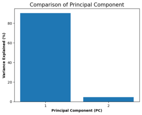
#checking the % of variance in price explained by the 2 components

percent_variance = np.round(pca.explained_variance_ratio_* 100, decimals =2)
columns = ['1', '2']
plt.bar(x= range(1,3), height=percent_variance, tick_label=columns)
plt.ylabel('Variance Explained (%)',fontweight='bold')
plt.xlabel('Principal Component (PC)',fontweight='bold')
plt.title('Comparison of Principal Component', size = 15)
plt.savefig('[Fig 4.5.1] PCA_Comparison of Principal Component.png', dpi = 300)
plt.show()

png

#scatter plot 

plt.scatter(principalDataframe.PC1, principalDataframe.PC2)
plt.title('PC1 against PC2',size = 15)
plt.xlabel('PC1')
plt.ylabel('PC2')
plt.savefig('[Fig 4.5.2] PCA_PC1 against PC2 Plot.png', dpi = 300)
plt.show()

png

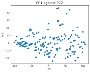
No significant pattern

pca.explained_variance_ratio_

array([0.90400936, 0.04652694])

Interpretation: These values show that the first principal component PC1 explains most of the variance in the target.
Decision: Build and visualizing the PCA model further. We will first disunite the train and test data and do the prediction.

def pca_dec(data, n):
  pca = PCA(n)
  princi_components = pca.fit_transform(data)
  return princi_components, pca

#Decomposing the train set:
X_trn_pca, pca_train = pca_dec(X_trn_new, 2)

#Decomposing the test set:
X_tst_pca, pca_test = pca_dec(X_tst_new, 2)

X_trn_df = pd.DataFrame(data = X_trn_pca, columns = ['X_trn_PC1', 'X_trn_PC2'])
print(X_trn_df.head())

X_tst_df = pd.DataFrame(data = X_tst_pca, columns = ['X_tst_PC1', 'X_tst_PC2'])
print(X_tst_df.head())

   X_trn_PC1  X_trn_PC2
49.980616  -9.744192
-61.296918  -7.668622
-47.127075  12.557807
-75.490579  -4.750386
 3.995841  -0.153073
   X_tst_PC1  X_tst_PC2
-63.997451  -0.032976
92.727444   6.319053
-88.593318   9.013806
-47.712789  -1.474157
27.551259  -8.689390

#fitting the model
lm.fit(X_trn_df,y_trn_new)

# predicting the test data
y_pred_pca = lm.predict(X_tst_df)

# checking the R2 score
linear_PCA_score = r2_score(y_tst_new,y_pred_pca)
linear_PCA_score

0.8638450042408081

Pickling The Model (Save and Load The Model)

with open('[4.5.1] PCA', 'wb') as f:
    pickle.dump(lm, f)
with open('[4.5.1] PCA', 'rb') as f:
    model_pca = pickle.load(f)
#testing the pickled model. reason: to make sure the pickle output showing the same as the current model (y_pred_pca)
model_pca.predict(X_tst_df)

array([ 37.9645029 , 172.52744095,  21.21491852,  51.03253584,
       111.1889147 ,  25.38711314, 173.82916435,  88.80386874,
       146.8090489 , 182.55372327, 166.16350822,  66.68738375,
       112.55506802,  79.55414464, 110.4527255 ,  55.12354572,
        84.5658018 ,  46.42722245,  81.73823254, 174.46440435,
       136.25278015, 175.67203409,  36.90366031,  35.08919826,
       170.70061726,  86.69380947,  90.77482424, 171.98816234,
       139.32298908, 131.17284191,  87.39179272,  21.05818118,
       101.22975087,  35.43966643,  61.7648987 , 133.13557043,
        52.79809295,  58.33223183, 110.25241132,  57.8805349 ,
       135.62780735, 143.60858845,  73.42031937,  33.8301877 ,
       131.5718391 , 137.31360752,  16.4349561 ,  26.01920097,
        93.35467871,  24.34346701, 153.7550102 , 145.27394444,
       101.56800115, 109.65780716,  31.527531  ,  26.22903964,
        82.97023874, 155.55407388,  92.6416299 ,  78.87094644,
        89.52036816,  76.56828975,  16.95296254, 123.42276321,
        40.21871637,  51.70121555,  75.64549286])

#Creating a table with the explained variance ratio for the train data set
names_pcas = [f"PCA Component {i}" for i in range(1, 3, 1)]
scree = pd.DataFrame(list(zip(names_pcas, pca_train.explained_variance_ratio_)), columns=["Component", "Explained Variance Ratio"])
print(scree)

         Component  Explained Variance Ratio
0  PCA Component 1                  0.896766
1  PCA Component 2                  0.048400

Interpretation: Based on the above it is conspicuous that PCA1 of the training dataset has availed expound virtually 90% of the variance in price (target), but we additionally need to find which of the features from the original dataset make up each of the components and which features contribute the highest to that eigenvectors.
Decision: Sorting the values of the first principal component by how large each one and sorting the absolute values of the first principal component by magnitude

#Sorting the values of the first principal component by how large each one is
df = pd.DataFrame({'PCA':pca_train.components_[0], 'Variable Names':list(X_trn_new.columns)})
df = df.sort_values('PCA', ascending=False)

#Sorting the absolute values of the first principal component by magnitude
df2 = pd.DataFrame(df)
df2['PCA']=df2['PCA'].apply(np.absolute)
df2 = df2.sort_values('PCA', ascending=False)
#print(df2['Variable Names'][0:11])

df.head()

	PCA	Variable Names
0	0.859986	curb_weight
1	0.329952	length
2	0.208613	horsepower
3	0.198711	wheel_base
5	0.166743	width

Interpretation: curb_weight is the most descriptive factor in PCA1 and contributes about 86% to PCA1, this makes an abundance of sense intuitively as the higher the curb weight the higher the other values are like length, width etc and hence is a significant factor in determining the price.

Model 6 - Final Iteration to Find Tune The PCA (Linear Regression Combo Model)

by using only those variables in the Linear Regression Model that make up the PCA1 components from above PCA Analysis.

# creating a data set to include only the components of the PCA1 above
X_PCA = x[['curb_weight', 'length','wheel_base','horsepower', 'width']].copy()

# training and splitting the data set
X_trn_PCA, X_tst_PCA, y_trn_PCA, y_tst_PCA = train_test_split(X_PCA, y, test_size=0.33, random_state=42)
print(X_trn_PCA.shape, X_tst_PCA.shape, y_trn_PCA.shape, y_tst_PCA.shape)

# scaling the data set
X_trn_PCA_fc = sc.fit_transform(X_trn_PCA)
X_tst_PCA_fc = sc.transform(X_tst_PCA)

#fitting the model
lm.fit(X_trn_PCA_fc,y_trn_PCA)

# predicting the test data
y_pred_PCA = lm.predict(X_tst_PCA_fc)

# checking the R2 score
linear_FinalRegrPCA_score = r2_score(y_tst_PCA,y_pred_PCA)
linear_FinalRegrPCA_score

(134, 5) (67, 5) (134,) (67,)

0.8812197638869728

Interpretation: The r2score has improved by using only the variables that make up the PCA1 component which betokens that these are the most consequential predictor variables to be considered for the car price prediction.

Pickling The Model (Save and Load The Model)

with open('[4.5.2] PCA (Linear Regression Combo Model)', 'wb') as f:
    pickle.dump(lm, f)
with open('[4.5.2] PCA (Linear Regression Combo Model)', 'rb') as f:
    model_pca = pickle.load(f)
#testing the pickled model. reason: to make sure the pickle output showing the same as the current model (y_pred_PCA)
model_pca.predict(X_tst_PCA_fc)

array([ 30.74360127, 173.57112374,  21.74652627,  43.45626682,
       112.35831945,  21.61600579, 169.22717335,  89.23820946,
       153.42475431, 183.79120412, 159.93260049,  59.56664013,
       108.70381117,  73.36807852, 112.60980703,  46.24767767,
        81.93197674,  40.43567559,  74.43145855, 178.32923086,
       132.54734325, 181.8906238 ,  27.03987554,  29.13324515,
       164.02119982,  75.95501644,  95.23767692, 169.33167933,
       134.56107074, 141.03022976,  86.53727535,  19.16285949,
       106.53860934,  30.50239658,  46.66850385, 128.32143598,
        38.30262547,  55.88322274, 107.19351556,  57.20532959,
       131.41269502, 145.88414287,  71.28145647,  27.15375637,
       129.04277478, 137.20080521,  11.23867913,  23.52419749,
        85.60234386,  22.08519895, 154.34938341, 152.41789056,
       103.85851436, 107.57552102,  25.64346075,  24.46121413,
        71.94949838, 150.96712485,  91.75536882,  78.01481834,
        83.26124916,  76.50452273,  14.49799789, 116.88844137,
        36.51338227,  40.63077699,  58.65781791])

png Image Credit

Summary of Analysis

# Summary of the Accuracy scores for test data

model_ev = pd.DataFrame({'Model': ['Linear Regression','Ridge Regression','Lasso Regression','SVR',
                    'PCA', 'PCA-Linear Combo'], 'r2 score (%)': [round(linear_FinalRegr_score*100, 3),
                    round(Ridge_RegrLn_Score*100, 3), round(Lasso_RegrLn_Score*100, 3),round(svr_r2_score*100, 3),round(linear_PCA_score*100, 3), round(linear_FinalRegrPCA_score*100, 3)]})

model_ev = model_ev.sort_values('r2 score (%)', ascending=False)

model_ev

	Model	r2 score (%)
5	PCA-Linear Combo	88.122
2	Lasso Regression	87.990
0	Linear Regression	87.983
1	Ridge Regression	87.983
3	SVR	86.440
4	PCA	86.385

#Bar plots of the r2scores for visualization

colors = ['red','green','blue','c','orange', 'yellow']
plt.figure(figsize=(15,7))
plt.title("Barplot of 6 Models", size = 15)
plt.xlabel("Models")
plt.xticks(rotation=0)
plt.ylim(86,88.5, 0.001)
plt.ylabel("r2 scores")
plt.bar(model_ev['Model'],model_ev['r2 score (%)'],color = colors)
plt.savefig('[Fig 5] Performance of Each Models', dpi = 300)
plt.show()

png

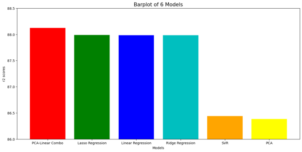
The most prominent model falls on PCA-Linear Regression Combo Model
Lasso - Ridge Regression models look identically tantamount (predicated on the graph above). However, speaking about the details, the digit precision of each r2 score needs to be considered.
Conclusion: PCA-Linear Regression Combo Model, it indicates better performance for predicting target (price).

Recommendation:

Lasso regression model is one of the best modeling techinque for this project. It also takes care of the multicollinearity issue that is present in this dataset without having to do any transformation of the dataset. It also takes less time in running compared to SVR.
The PCA Analysis took care of most of the multicollinearity issues and provided us 5 predictor variables (curb weight, length, horse power, wheel base and width) that can accurately predict the car prices. The Linear Regression model with these 5 predictor variables gave the best r2score and so we recommend the usage of this PCA-Linear Regression Model for this project.

Project Risks

We have taken the 10 best features from the feature selection algorithm to reduce the dimensionality problem for modeling purposes, so if there are any interaction effects between the features that have not been modeled, due to lack of expertise in this field, there may be considerable amount of underperformance in the model when it is implemented.

The project postulates that the dataset utilized for modeling in this project is a representative of the population dataset else the models may not provide the accuracies that are shown here.

← Previous Post Next Post →

	symboling	normalized_losses	make	fuel_type	num_of_doors	body_style	drive_wheels	wheel_base	...	engine_size	fuel_system	bore	stroke	compression_ratio	horsepower	peak_rpm	city_mpg	highway_mpg	price
0	5	28	0	1	1	0	2	2	...	18	5	24	4	13	31	10	8	10	117
1	5	28	0	1	1	0	2	2	...	18	5	24	4	13	31	10	8	10	136
2	3	28	0	1	1	2	2	10	...	28	5	1	28	13	46	10	6	9	136
3	4	42	1	1	0	3	1	29	...	11	5	13	25	22	27	17	11	13	122
4	4	42	1	1	0	3	0	28	...	22	5	13	25	5	34	17	5	5	147

	curb_weight	length	horsepower	wheel_base	height	engine_size	normalized_losses	width	bore	stroke
0	92	22	31	2	1	18	28	8	24	4
1	92	22	31	2	1	18	28	8	24	4
2	115	29	46	10	13	28	28	16	1	28
3	66	44	27	29	25	11	42	21	13	25
4	116	44	34	28	25	22	42	23	13	25

	curb_weight	length	horsepower	wheel_base	height	engine_size	normalized_losses	width	bore	stroke	price
0	92	22	31	2	1	18	28	8	24	4	117
1	92	22	31	2	1	18	28	8	24	4	136
2	115	29	46	10	13	28	28	16	1	28	136
3	66	44	27	29	25	11	42	21	13	25	122
4	116	44	34	28	25	22	42	23	13	25	147

	curb_weight	length	horsepower	wheel_base	engine_size	width	bore
0	92	22	31	2	18	8	24
1	92	22	31	2	18	8	24
2	115	29	46	10	28	16	1
3	66	44	27	29	11	21	13
4	116	44	34	28	22	23	13

	symboling	normalized_losses	make	fuel_type	num_of_doors	body_style	drive_wheels	wheel_base	...	engine_size	fuel_system	bore	stroke	compression_ratio	horsepower	peak_rpm	city_mpg	highway_mpg	price
0	5	28	0	1	1	0	2	2	...	18	5	24	4	13	31	10	8	10	117
1	5	28	0	1	1	0	2	2	...	18	5	24	4	13	31	10	8	10	136
2	3	28	0	1	1	2	2	10	...	28	5	1	28	13	46	10	6	9	136
3	4	42	1	1	0	3	1	29	...	11	5	13	25	22	27	17	11	13	122
4	4	42	1	1	0	3	0	28	...	22	5	13	25	5	34	17	5	5	147

	curb_weight	length	horsepower	wheel_base	height	engine_size	normalized_losses	width	bore	stroke
0	92	22	31	2	1	18	28	8	24	4
1	92	22	31	2	1	18	28	8	24	4
2	115	29	46	10	13	28	28	16	1	28
3	66	44	27	29	25	11	42	21	13	25
4	116	44	34	28	25	22	42	23	13	25

	curb_weight	length	horsepower	wheel_base	height	engine_size	normalized_losses	width	bore	stroke	price
0	92	22	31	2	1	18	28	8	24	4	117
1	92	22	31	2	1	18	28	8	24	4	136
2	115	29	46	10	13	28	28	16	1	28	136
3	66	44	27	29	25	11	42	21	13	25	122
4	116	44	34	28	25	22	42	23	13	25	147

	curb_weight	length	horsepower	wheel_base	engine_size	width	bore
0	92	22	31	2	18	8	24
1	92	22	31	2	18	8	24
2	115	29	46	10	28	16	1
3	66	44	27	29	11	21	13
4	116	44	34	28	22	23	13

	symboling	normalized_losses	make	fuel_type	num_of_doors	body_style	drive_wheels	wheel_base	...	engine_size	fuel_system	bore	stroke	compression_ratio	horsepower	peak_rpm	city_mpg	highway_mpg	price
0	5	28	0	1	1	0	2	2	...	18	5	24	4	13	31	10	8	10	117
1	5	28	0	1	1	0	2	2	...	18	5	24	4	13	31	10	8	10	136
2	3	28	0	1	1	2	2	10	...	28	5	1	28	13	46	10	6	9	136
3	4	42	1	1	0	3	1	29	...	11	5	13	25	22	27	17	11	13	122
4	4	42	1	1	0	3	0	28	...	22	5	13	25	5	34	17	5	5	147

	curb_weight	length	horsepower	wheel_base	height	engine_size	normalized_losses	width	bore	stroke
0	92	22	31	2	1	18	28	8	24	4
1	92	22	31	2	1	18	28	8	24	4
2	115	29	46	10	13	28	28	16	1	28
3	66	44	27	29	25	11	42	21	13	25
4	116	44	34	28	25	22	42	23	13	25

	curb_weight	length	horsepower	wheel_base	height	engine_size	normalized_losses	width	bore	stroke	price
0	92	22	31	2	1	18	28	8	24	4	117
1	92	22	31	2	1	18	28	8	24	4	136
2	115	29	46	10	13	28	28	16	1	28	136
3	66	44	27	29	25	11	42	21	13	25	122
4	116	44	34	28	25	22	42	23	13	25	147

	curb_weight	length	horsepower	wheel_base	engine_size	width	bore
0	92	22	31	2	18	8	24
1	92	22	31	2	18	8	24
2	115	29	46	10	28	16	1
3	66	44	27	29	11	21	13
4	116	44	34	28	22	23	13