Cellphone Price Prediction

Project Team ID = PTID-CDS-JUL21-1171 (Members - Diana, Hema, Pavithra and Sophiya)

Project ID = PRCP-1009-CellphonePrice (Cellphone Price Range)

Phase 1: Loading the Dataset and Understanding The Difference Features and Target

import numpy as np
%matplotlib inline
import pandas as pd
import matplotlib.pyplot as plt
import seaborn as sns
import warnings
warnings.filterwarnings("ignore")

data =  pd.read_csv('datasets_11167_15520_train.csv')

data.head()

	battery_power	blue	clock_speed	dual_sim	fc	four_g	int_memory	m_dep	mobile_wt	n_cores	...	px_height	px_width	ram	sc_h	sc_w	talk_time	three_g	touch_screen	wifi	price_range
0	842	0	2.2	0	1	0	7	0.6	188	2	...	20	756	2549	9	7	19	0	0	1	1
1	1021	1	0.5	1	0	1	53	0.7	136	3	...	905	1988	2631	17	3	7	1	1	0	2
2	563	1	0.5	1	2	1	41	0.9	145	5	...	1263	1716	2603	11	2	9	1	1	0	2
3	615	1	2.5	0	0	0	10	0.8	131	6	...	1216	1786	2769	16	8	11	1	0	0	2
4	1821	1	1.2	0	13	1	44	0.6	141	2	...	1208	1212	1411	8	2	15	1	1	0	1

5 rows × 21 columns

Description of the Dataset

battery_power:Total energy a battery can store in one time measured in mAh

blue:Has bluetooth or not

clock_speed:speed at which microprocessor executes instructions

dual_sim:Has dual sim support or not

fc:Front Camera mega pixels

four_g:Has 4G or not

int_memory:Internal Memory in Gigabytes

m_dep:Mobile Depth in cm

mobile_wt:Weight of mobile phone

n_cores:Number of cores of processor

pc:Primary Camera mega pixels

px_height:Pixel Resolution Height

px_width:Pixel Resolution Width

ram:Random Access Memory in Megabytes

sc_h:Screen Height of mobile in cm

sc_w:Screen Width of mobile in cm

talk_time:longest time that a single battery charge will last when you are

three_g:Has 3G or not

touch_screen:Has touch screen or not

wifi:Has wifi or not

price_range: three classifications could be high range, mid range and low range (dont know how the target is scaled)

print("____________________________________________")
print("            Info of The Dataset")
print("____________________________________________")
data.info() 

____________________________________________
            Info of The Dataset
____________________________________________
<class 'pandas.core.frame.DataFrame'>
RangeIndex: 2000 entries, 0 to 1999
Data columns (total 21 columns):
 #   Column         Non-Null Count  Dtype  
---  ------         --------------  -----  
 0   battery_power  2000 non-null   int64  
 1   blue           2000 non-null   int64  
 2   clock_speed    2000 non-null   float64
 3   dual_sim       2000 non-null   int64  
 4   fc             2000 non-null   int64  
 5   four_g         2000 non-null   int64  
 6   int_memory     2000 non-null   int64  
 7   m_dep          2000 non-null   float64
 8   mobile_wt      2000 non-null   int64  
 9   n_cores        2000 non-null   int64  
 10  pc             2000 non-null   int64  
 11  px_height      2000 non-null   int64  
 12  px_width       2000 non-null   int64  
 13  ram            2000 non-null   int64  
 14  sc_h           2000 non-null   int64  
 15  sc_w           2000 non-null   int64  
 16  talk_time      2000 non-null   int64  
 17  three_g        2000 non-null   int64  
 18  touch_screen   2000 non-null   int64  
 19  wifi           2000 non-null   int64  
 20  price_range    2000 non-null   int64  
dtypes: float64(2), int64(19)
memory usage: 328.2 KB

data.isnull().sum()

battery_power    0
blue             0
clock_speed      0
dual_sim         0
fc               0
four_g           0
int_memory       0
m_dep            0
mobile_wt        0
n_cores          0
pc               0
px_height        0
px_width         0
ram              0
sc_h             0
sc_w             0
talk_time        0
three_g          0
touch_screen     0
wifi             0
price_range      0
dtype: int64

data.describe().T

	count	mean	std	min	25%	50%	75%	max
battery_power	2000.0	1238.51850	439.418206	501.0	851.75	1226.0	1615.25	1998.0
blue	2000.0	0.49500	0.500100	0.0	0.00	0.0	1.00	1.0
clock_speed	2000.0	1.52225	0.816004	0.5	0.70	1.5	2.20	3.0
dual_sim	2000.0	0.50950	0.500035	0.0	0.00	1.0	1.00	1.0
fc	2000.0	4.30950	4.341444	0.0	1.00	3.0	7.00	19.0
four_g	2000.0	0.52150	0.499662	0.0	0.00	1.0	1.00	1.0
int_memory	2000.0	32.04650	18.145715	2.0	16.00	32.0	48.00	64.0
m_dep	2000.0	0.50175	0.288416	0.1	0.20	0.5	0.80	1.0
mobile_wt	2000.0	140.24900	35.399655	80.0	109.00	141.0	170.00	200.0
n_cores	2000.0	4.52050	2.287837	1.0	3.00	4.0	7.00	8.0
pc	2000.0	9.91650	6.064315	0.0	5.00	10.0	15.00	20.0
px_height	2000.0	645.10800	443.780811	0.0	282.75	564.0	947.25	1960.0
px_width	2000.0	1251.51550	432.199447	500.0	874.75	1247.0	1633.00	1998.0
ram	2000.0	2124.21300	1084.732044	256.0	1207.50	2146.5	3064.50	3998.0
sc_h	2000.0	12.30650	4.213245	5.0	9.00	12.0	16.00	19.0
sc_w	2000.0	5.76700	4.356398	0.0	2.00	5.0	9.00	18.0
talk_time	2000.0	11.01100	5.463955	2.0	6.00	11.0	16.00	20.0
three_g	2000.0	0.76150	0.426273	0.0	1.00	1.0	1.00	1.0
touch_screen	2000.0	0.50300	0.500116	0.0	0.00	1.0	1.00	1.0
wifi	2000.0	0.50700	0.500076	0.0	0.00	1.0	1.00	1.0
price_range	2000.0	1.50000	1.118314	0.0	0.75	1.5	2.25	3.0

data['price_range'].value_counts()

  500
  500
  500
  500
Name: price_range, dtype: int64

Teams Remarks: Data seems to be balanced for each of the classes with no null values for any of the variables

Phase 2: Data Preparation

from sklearn.preprocessing import  LabelEncoder

# ENCODING THE ENTIRE DATA SET
label = LabelEncoder()
data1 = data.apply(label.fit_transform)
data1

	battery_power	blue	clock_speed	dual_sim	fc	four_g	int_memory	m_dep	mobile_wt	n_cores	...	px_height	px_width	ram	sc_h	sc_w	talk_time	three_g	touch_screen	wifi	price_range
0	255	0	17	0	1	0	5	5	108	1	...	18	186	963	4	7	17	0	0	1	1
1	382	1	0	1	0	1	51	6	56	2	...	738	1099	998	12	3	5	1	1	0	2
2	48	1	0	1	2	1	39	8	65	4	...	962	901	984	6	2	7	1	1	0	2
3	88	1	20	0	0	0	8	7	51	5	...	935	954	1055	11	8	9	1	0	0	2
4	954	1	7	0	13	1	42	5	61	1	...	928	517	499	3	2	13	1	1	0	1
...	...	...	...	...	...	...	...	...	...	...	...	...	...	...	...	...	...	...	...	...	...
1995	216	1	0	1	0	1	0	7	26	5	...	939	1022	180	8	4	17	1	1	0	0
1996	1064	1	21	1	0	0	37	1	107	3	...	745	1080	732	6	10	14	1	1	1	2
1997	1027	0	4	1	1	1	34	6	28	7	...	716	834	1158	4	1	3	1	1	0	3
1998	732	0	4	0	4	1	44	0	65	4	...	283	120	266	13	10	17	1	1	1	0
1999	8	1	15	1	5	1	43	8	88	5	...	413	184	1526	14	4	0	1	1	1	3

2000 rows × 21 columns

# splitting the data into X and Y so we can do feature selection

x  = data1.drop('price_range', axis=1)
y = data1['price_range']
print(x.head())
y.head()

   battery_power  blue  clock_speed  dual_sim  fc  four_g  int_memory  m_dep  \
          255     0           17         0   1       0           5      5   
          382     1            0         1   0       1          51      6   
           48     1            0         1   2       1          39      8   
           88     1           20         0   0       0           8      7   
          954     1            7         0  13       1          42      5   

   mobile_wt  n_cores  pc  px_height  px_width   ram  sc_h  sc_w  talk_time  \
      108        1   2         18       186   963     4     7         17   
       56        2   6        738      1099   998    12     3          5   
       65        4   6        962       901   984     6     2          7   
       51        5   9        935       954  1055    11     8          9   
       61        1  14        928       517   499     3     2         13   

   three_g  touch_screen  wifi  
      0             0     1  
      1             1     0  
      1             1     0  
      1             0     0  
      1             1     0  





  1
  2
  2
  2
  1
Name: price_range, dtype: int64

Too much input variables will be decreasing the accuracy of models so using the feature selection technique to reduce the no. of input variables that contribute less to predicting the target

# FEATURE SELECTION TECHNIQUE

from sklearn.feature_selection import SelectKBest
from sklearn.feature_selection import chi2

#apply SelectKBest class to extract top 10 best features
bestfeatures = SelectKBest(score_func=chi2, k=10)
fit = bestfeatures.fit(x,y)
dfscores = pd.DataFrame(fit.scores_)
dfcolumns = pd.DataFrame(x.columns)

#concat two dataframes for better visualization
featurescores = pd.concat([dfcolumns,dfscores], axis=1)
featurescores.columns = ['Specs', 'Score'] #naming the data
print(featurescores.nlargest(10, 'Score'))

            Specs          Score
          ram  428852.649505
 battery_power   16835.196948
     px_width   12243.820689
    px_height    9989.550625
     mobile_wt     223.407824
    int_memory      95.819130
         sc_w      16.480319
         sc_h      16.194553
    talk_time      16.174231
       n_cores      11.681721

The top 10 features are now used to build the models for comparison

Modifying the dataset to include only these 10 important features

X = x[['ram', 'battery_power', 'px_width','px_height','mobile_wt','int_memory','sc_w','sc_h','talk_time','n_cores']].copy()

X.head()

	ram	battery_power	px_width	px_height	mobile_wt	int_memory	sc_w	sc_h	talk_time	n_cores
0	963	255	186	18	108	5	7	4	17	1
1	998	382	1099	738	56	51	3	12	5	2
2	984	48	901	962	65	39	2	6	7	4
3	1055	88	954	935	51	8	8	11	9	5
4	499	954	517	928	61	42	2	3	13	1

Phase 3: Exploratory Data Analysis

# Checking for the skewness and kurtosis for 10 selected features and target

print("Skewness of ram: %f" %X['ram'].skew())
print("Kurtosis of ram: %f" %X['ram'].kurt())
print("Skewness of battery power: %f" %X['battery_power'].skew())
print("Kurtosis of battery power: %f" %X['battery_power'].kurt())
print("Skewness of Pixel Width: %f" %X['px_width'].skew())
print("Kurtosis of Pixel Width: %f" %X['px_width'].kurt())
print("Skewness of Pixel Height: %f" %X['px_height'].skew())
print("Kurtosis of Pixel Height: %f" %X['px_height'].kurt())
print("Skewness of Mobile Weight: %f" %X['mobile_wt'].skew())
print("Kurtosis of Mobile Weight: %f" %X['mobile_wt'].kurt())
print("Skewness of Internal Memory: %f" %X['int_memory'].skew())
print("Kurtosis of Internal Memory: %f" %X['int_memory'].kurt())
print("Skewness of Screen Width: %f" %X['sc_w'].skew())
print("Kurtosis of Screen Width: %f" %X['sc_w'].kurt())
print("Skewness of Screen Height: %f" %X['sc_h'].skew())
print("Kurtosis of Screen Height: %f" %X['sc_h'].kurt())
print("Skewness of Talking Time Performance: %f" %X['talk_time'].skew())
print("Kurtosis of Talking Time Performance: %f" %X['talk_time'].kurt())
print("Skewness of Number Cores Processor: %f" %X['n_cores'].skew())
print("Kurtosis of Number Cores Processor: %f" %X['n_cores'].kurt())
print("Skewness of Price Range: %f" %data1['price_range'].skew())
print("Kurtosis of Price Range: %f" %data1['price_range'].kurt())

Skewness of ram: -0.001103
Kurtosis of ram: -1.171483
Skewness of battery power: 0.028115
Kurtosis of battery power: -1.206078
Skewness of Pixel Width: 0.029001
Kurtosis of Pixel Width: -1.198770
Skewness of Pixel Height: 0.237204
Kurtosis of Pixel Height: -1.090681
Skewness of Mobile Weight: 0.006558
Kurtosis of Mobile Weight: -1.210376
Skewness of Internal Memory: 0.057889
Kurtosis of Internal Memory: -1.216074
Skewness of Screen Width: 0.633787
Kurtosis of Screen Width: -0.389523
Skewness of Screen Height: -0.098884
Kurtosis of Screen Height: -1.190791
Skewness of Talking Time Performance: 0.009512
Kurtosis of Talking Time Performance: -1.218591
Skewness of Number Cores Processor: 0.003628
Kurtosis of Number Cores Processor: -1.229750
Skewness of Price Range: 0.000000
Kurtosis of Price Range: -1.360400

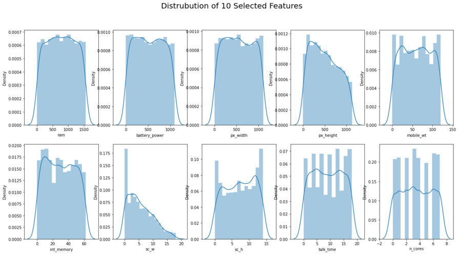
Reference - Skewness between -0.5 and 0.5: data fairly symmetrical. Skewness between -1 and – 0.5 or between 0.5 and 1: data moderately skewed. Skewness is less than -1 or greater than 1: the data are highly skewed. Kurtosis bettween -2 and +2 are considered acceptable.

Teams Remarks: The Skewness and Kurtosis for all the predictor and target variables falls within the acceptable range.

figure, ax = plt.subplots(2,5, figsize=(20,10))

#See the distrubution of the data
plt.suptitle('Distrubution of 10 Selected Features', size = 20)
sns.distplot(data1['ram'],ax=ax[0,0])
sns.distplot(data1['battery_power'], ax=ax[0,1])
sns.distplot(data1['px_width'], ax=ax[0,2])
sns.distplot(data1['px_height'], ax=ax[0,3])
sns.distplot(data1['mobile_wt'], ax=ax[0,4])
sns.distplot(data1['int_memory'], ax=ax[1,0])
sns.distplot(data1['sc_w'], ax=ax[1,1])
sns.distplot(data1['sc_h'], ax=ax[1,2])
sns.distplot(data1['talk_time'], ax=ax[1,3])
sns.distplot(data1['n_cores'], ax=ax[1,4])
plt.savefig('EDA - Distplot Visualization.png', dpi = 300)
plt.show()

png

#slicing 10 selected features to display boxplot. reasons to do that: the range of some features are different
slice_X1 = X[['ram', 'battery_power', 'px_width', 'px_height', 'mobile_wt']]
slice_X1
slice_X2 = X[['int_memory', 'sc_w', 'sc_h', 'talk_time', 'n_cores']]
slice_X2

	int_memory	sc_w	sc_h	talk_time	n_cores
0	5	7	4	17	1
1	51	3	12	5	2
2	39	2	6	7	4
3	8	8	11	9	5
4	42	2	3	13	1
...	...	...	...	...	...
1995	0	4	8	17	5
1996	37	10	6	14	3
1997	34	1	4	3	7
1998	44	10	13	17	4
1999	43	4	14	0	5

2000 rows × 5 columns

#Boxplot to check any outlier
plt.figure(figsize=(20,15))
plt.subplot(2, 2, 1)
sns.set_theme(style="darkgrid")
ax = sns.boxplot(data=slice_X1, orient="w", palette="Dark2")
plt.subplot(2, 2, 2)
sns.set_theme(style="darkgrid")
ax = sns.boxplot(data=slice_X2, orient="w", palette="Dark2_r")
plt.suptitle("Boxplot of of 10 Selected Features", size = 25)
plt.savefig('EDA - Boxplot Visualization.png', dpi = 300)
plt.show()
print('Checking...========================================\nResult: Outliers Not Found')

png

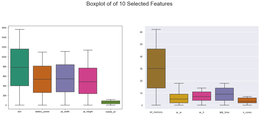
Checking...========================================
Result: Outliers Not Found

No significant outliers in the dataset

#combining the x (features) and y (target) to show the heatmap and pairplot analysis

xydata = data1[['ram', 'battery_power', 'px_width','px_height','mobile_wt','int_memory','sc_w','sc_h','talk_time','n_cores', 'price_range']].copy()

xydata.head()

	ram	battery_power	px_width	px_height	mobile_wt	int_memory	sc_w	sc_h	talk_time	n_cores	price_range
0	963	255	186	18	108	5	7	4	17	1	1
1	998	382	1099	738	56	51	3	12	5	2	2
2	984	48	901	962	65	39	2	6	7	4	2
3	1055	88	954	935	51	8	8	11	9	5	2
4	499	954	517	928	61	42	2	3	13	1	1

#Heatmap to shows the correlation
plt.figure(figsize=(20,15))
sns.heatmap(xydata.corr(),cmap='nipy_spectral',annot=True)
plt.title('Heatmap Shows The Relationship (correlation) Between Selected Features',
         fontsize=25)
plt.savefig('EDA - Heatmap Visualization.png', dpi = 300)
plt.show()

png

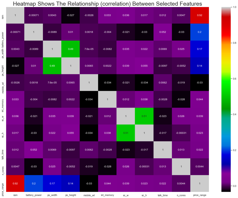
Teams Remarks: Ram dictates 92% of the price range classification. Screen width and screen height seem to be correlated, so we may merge them to reduce any dimensionality problems. For now we have decided to leave it in there for modelling purposes. No other major collinearlity issues

#pairplot analysis

sns.pairplot(xydata, hue = 'price_range', corner=True, palette='gnuplot')
plt.savefig('EDA - Pairplot Visualization.png', dpi = 300)
plt.show()

png

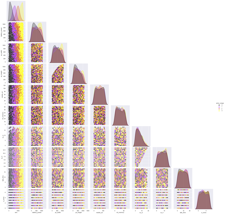
Teams remarks: As is evident from the pair plots, ram is going to be a significant variable to determine the decision boundaries for the models

#checking to see y counts

y.value_counts()

  500
  500
  500
  500
Name: price_range, dtype: int64

Phase 4: Modelling Strategy

Given this is a classification problem for multiple classes, several models will be used for the comparitive analysis and the best model will be chosen for this project

Model 1: K Means

Model 2: KNN

Model 3: Decision Tree

Model 4: Random Forest

Model 5: XG Boost

Model 6: SVM Classification

Splitting the dataset into train and test data sets for validation

from sklearn.model_selection import train_test_split
X_train, X_test, y_train, y_test = train_test_split(X, y, test_size=0.33, random_state=42, stratify=y) #stratify -> it can reduce the variability of sample statistics
X_train.shape, X_test.shape, y_train.shape, y_test.shape

((1340, 10), (660, 10), (1340,), (660,))

Scaling the train and test datasets

#feature scaling
from sklearn.preprocessing import StandardScaler
sc = StandardScaler()
X_train_fc = sc.fit_transform(X_train)
X_test_fc = sc.transform(X_test)

Model 1: K Means

from sklearn.model_selection import GridSearchCV

from sklearn.cluster import KMeans

# Model building

kmeans_mod = KMeans()

kmeans_mod = KMeans(n_clusters = 4, random_state = 0)
kmeans_mod.fit(X)
kmeans_mod.labels_

array([1, 0, 0, ..., 0, 3, 1])

from datetime import datetime
start_time = datetime.now()

from datetime import timedelta

start = timeit.default_timer()
kmeans_mod = KMeans()
kmeans_mod = KMeans(n_clusters = 4, random_state = 0)
kmeans_mod.fit(X)
kmeans_mod.labels_
kmeans_mod.predict(X)
clusters = kmeans_mod.labels_
Kmeansscore = silhouette_score(X, clusters, metric='euclidean')
Kmeansscore
stop = timeit.default_timer()
execution_time = stop - start
print("Program Executed in "+str(execution_time), 'seconds') # It returns time in seconds
#print(timedelta(seconds=end_time - start_time))
#print('Duration: {}'.format(end_time - start_time))

Program Executed in 0.35800029999995786 seconds

start = timeit.default_timer()
kmeans_mod = KMeans()
kmeans_mod = KMeans(n_clusters = 4, random_state = 0)
kmeans_mod.fit(X)
kmeans_mod.labels_
kmeans_mod.predict(X)
clusters = kmeans_mod.labels_
Kmeansscore = silhouette_score(X, clusters, metric='euclidean')
Kmeansscore
stop = timeit.default_timer()
execution_time = stop - start
print("Program Executed in "+str(round(execution_time, 2)), 'seconds') # It returns time in seconds
#print(timedelta(seconds=end_time - start_time))
#print('Duration: {}'.format(end_time - start_time))

Program Executed in 0.39 seconds

#scatterplot analysis

sns.scatterplot(x = 'ram', y = 'battery_power', data = X, hue=y, style= kmeans_mod.labels_, palette=['orange', 'blue', 'red', 'green'])
plt.scatter(kmeans_mod.cluster_centers_[:, 0], kmeans_mod.cluster_centers_[:,1], marker='X', s=200, c='red')
plt.savefig('KMeans Scatterplot.png', dpi = 300)
plt.show()

png

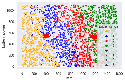
Teams Remarks: Data seems to be overlapping quite a bit at the boundaries (no clear and distinct boundaries) so K Means does not do well in such scenarios as the neighbours are mingled near the boundaries

kmeans_mod.predict(X)

array([1, 0, 0, ..., 0, 3, 1])

#checking the model score
from sklearn.metrics import silhouette_score
clusters = kmeans_mod.labels_
Kmeansscore = silhouette_score(X, clusters, metric='euclidean')
Kmeansscore

0.22549709096550374

Pickling The Model (Save and Load The Model)

import pickle

with open('kmeans_pickle', 'wb') as f:
    pickle.dump(kmeans_mod, f)

with open('kmeans_pickle', 'rb') as f:
    model_kmeans = pickle.load(f)

model_kmeans.predict(X) #testing the model. reason: to make sure the pickle output showing the same as the current model

array([1, 0, 0, ..., 0, 3, 1])

Teams Remarks: As expected the silhouette score is very low indicating that this modelling technique is not apt for this project __ __

Model 2: KNN

from sklearn.neighbors import KNeighborsClassifier
from sklearn.metrics import confusion_matrix,  accuracy_score, classification_report

# Model building

knn = KNeighborsClassifier() 

# Search parameters
param = range(75, 200, 2)

# Sets up GridSearchCV object and stores it in grid variable
grid = GridSearchCV(knn,{'n_neighbors': param})

# Fits the grid object and gets the best model
best_knn = grid.fit(X_train,y_train).best_estimator_

# Displays the optimum model
best_knn

KNeighborsClassifier(n_neighbors=93)

Grid search found the optimal k value to be 93, using that for the final model below and testing for accuracy

knn = KNeighborsClassifier(n_neighbors=93)
knn.fit(X_train, y_train)
knn_predicted = knn.predict(X_test)
knn_conf_matrix = confusion_matrix(y_test, knn_predicted)
knn_acc_score = accuracy_score(y_test, knn_predicted)
print("confusion matrix")
print(knn_conf_matrix)
print("-------------------------------------------")
print("Accuracy of K-NeighborsClassifier:",knn_acc_score*100,'\n')
print("-------------------------------------------")
print(classification_report(y_test,knn_predicted))

confusion matrix
[[155  10   0   0]
 [  3 154   8   0]
 [  0  11 145   9]
 [  0   0  19 146]]
-------------------------------------------
Accuracy of K-NeighborsClassifier: 90.9090909090909 

-------------------------------------------
              precision    recall  f1-score   support

           0       0.98      0.94      0.96       165
           1       0.88      0.93      0.91       165
           2       0.84      0.88      0.86       165
           3       0.94      0.88      0.91       165

    accuracy                           0.91       660
   macro avg       0.91      0.91      0.91       660
weighted avg       0.91      0.91      0.91       660

# prediction

knn_train_predict  = knn.predict(X_train)
knn_test_predict   = knn.predict(X_test)

# training and testing accuracy scores

print(accuracy_score(y_train ,knn_train_predict))
KNNscore = accuracy_score(y_test ,knn_test_predict)
KNNscore

9097014925373135

9090909090909091

Pickling The Model (Save and Load The Model)

with open('knn_pickle', 'wb') as f:
    pickle.dump(knn, f)

with open('knn_pickle', 'rb') as f:
    model_knn = pickle.load(f)

model_knn.predict(X_test) #testing the model. reason: to make sure the pickle output showing the same as the current model

array([0, 1, 3, 3, 1, 3, 3, 1, 2, 2, 3, 3, 2, 1, 0, 3, 2, 0, 3, 3, 0, 2,
       1, 1, 3, 3, 1, 0, 1, 3, 3, 1, 3, 3, 1, 2, 3, 1, 3, 3, 2, 2, 2, 3,
       2, 2, 2, 0, 3, 0, 0, 2, 0, 3, 1, 0, 1, 3, 2, 1, 0, 2, 2, 1, 0, 2,
       0, 2, 0, 0, 1, 2, 3, 1, 1, 0, 2, 1, 1, 3, 2, 1, 0, 1, 3, 1, 2, 0,
       0, 0, 0, 3, 3, 0, 2, 1, 3, 2, 3, 1, 0, 2, 2, 0, 0, 3, 2, 2, 1, 0,
       3, 2, 1, 1, 0, 1, 2, 3, 3, 2, 1, 0, 1, 0, 3, 2, 0, 0, 0, 2, 3, 1,
       2, 0, 1, 0, 2, 1, 0, 2, 1, 1, 3, 2, 3, 2, 3, 0, 3, 1, 2, 1, 2, 1,
       2, 0, 0, 1, 3, 3, 2, 2, 2, 0, 2, 2, 1, 0, 1, 2, 3, 2, 0, 3, 3, 1,
       1, 0, 1, 2, 1, 0, 2, 2, 1, 3, 2, 0, 2, 3, 3, 0, 1, 2, 2, 2, 3, 1,
       3, 0, 2, 2, 0, 3, 1, 1, 1, 3, 1, 2, 2, 1, 3, 2, 2, 3, 3, 2, 2, 0,
       1, 0, 3, 3, 3, 2, 0, 1, 3, 1, 3, 0, 3, 2, 0, 0, 2, 1, 0, 2, 0, 2,
       0, 1, 3, 3, 2, 0, 1, 1, 0, 0, 3, 0, 3, 2, 3, 1, 1, 1, 1, 1, 3, 1,
       0, 1, 0, 1, 1, 3, 1, 1, 2, 3, 3, 1, 2, 3, 2, 2, 1, 1, 1, 2, 1, 1,
       0, 3, 0, 3, 2, 1, 1, 3, 0, 2, 3, 0, 0, 0, 2, 1, 1, 2, 2, 3, 1, 1,
       1, 1, 0, 0, 1, 1, 2, 2, 2, 0, 2, 0, 2, 3, 3, 0, 2, 3, 0, 2, 3, 2,
       1, 0, 1, 2, 2, 0, 1, 0, 1, 0, 0, 2, 3, 3, 1, 2, 2, 0, 0, 2, 3, 1,
       2, 2, 3, 2, 2, 3, 1, 0, 0, 3, 0, 3, 0, 0, 0, 3, 1, 3, 3, 2, 1, 1,
       1, 3, 0, 1, 1, 1, 1, 3, 0, 1, 1, 2, 0, 0, 2, 0, 2, 1, 2, 3, 2, 3,
       1, 2, 3, 0, 3, 3, 0, 3, 0, 0, 0, 3, 0, 0, 1, 0, 1, 0, 2, 2, 1, 0,
       2, 3, 1, 2, 3, 2, 3, 1, 3, 3, 2, 2, 2, 3, 1, 3, 2, 0, 3, 2, 0, 1,
       0, 2, 3, 0, 0, 0, 1, 0, 0, 1, 2, 1, 0, 1, 1, 2, 1, 2, 1, 1, 0, 1,
       3, 3, 0, 0, 1, 3, 2, 3, 3, 1, 1, 3, 1, 2, 1, 3, 2, 0, 2, 0, 1, 1,
       1, 3, 1, 3, 3, 1, 3, 2, 3, 3, 2, 1, 3, 2, 2, 3, 0, 1, 1, 0, 0, 2,
       2, 1, 1, 1, 3, 0, 0, 2, 3, 2, 2, 1, 1, 0, 1, 1, 0, 0, 1, 3, 2, 2,
       3, 1, 0, 1, 0, 0, 0, 0, 3, 1, 3, 3, 1, 0, 0, 1, 2, 2, 3, 0, 2, 1,
       2, 3, 2, 0, 1, 3, 2, 2, 3, 3, 3, 1, 3, 3, 2, 2, 1, 2, 0, 0, 0, 1,
       0, 3, 2, 0, 0, 2, 1, 0, 1, 0, 1, 3, 3, 0, 2, 3, 1, 0, 1, 3, 1, 2,
       2, 2, 0, 2, 3, 3, 3, 2, 2, 2, 2, 0, 2, 1, 3, 2, 1, 3, 2, 0, 2, 2,
       2, 3, 1, 1, 0, 3, 1, 3, 2, 1, 0, 1, 1, 2, 3, 0, 3, 0, 2, 0, 0, 0,
       1, 0, 1, 2, 3, 1, 0, 3, 0, 2, 2, 2, 2, 0, 2, 1, 1, 3, 2, 1, 1, 0],
      dtype=int64)

Model 3: Decision Tree

# Model building

from sklearn.tree import DecisionTreeClassifier
Deci_Tree_model  = DecisionTreeClassifier()

parameters = {'max_depth':[3,5,10,20,30],
              'random_state': [0,1,2,3,4] 
             }  

grid = GridSearchCV(Deci_Tree_model,parameters,cv=5,verbose=1) 
grid.fit(X_train,y_train)

Fitting 5 folds for each of 25 candidates, totalling 125 fits

GridSearchCV(cv=5, estimator=DecisionTreeClassifier(),
             param_grid={'max_depth': [3, 5, 10, 20, 30],
                         'random_state': [0, 1, 2, 3, 4]},
             verbose=1)

# printing best parameters from the above grid analysis

print(grid.best_params_)

{'max_depth': 10, 'random_state': 3}

Grid search has provided the best parameters for the tree, so using these parameters for the final tree below, the depth of 10 seems to be ok given there are 10 predictor variables

# Model building

Deci_Tree_best_model  = DecisionTreeClassifier(max_depth=10, random_state=3)

# Model fitting to the datasets

Deci_Tree_best_model.fit(X_train , y_train)

DecisionTreeClassifier(max_depth=10, random_state=3)

# Training and testing of the model

train_predict  = Deci_Tree_best_model.predict(X_train)
test_predict   = Deci_Tree_best_model.predict(X_test)

# checking the accuracy scores of the model

Deci_Tree_train_accuracyscore = accuracy_score(y_train ,train_predict)
Deci_Tree_test_accuracyscore = accuracy_score(y_test, test_predict)
print(Deci_Tree_train_accuracyscore, Deci_Tree_test_accuracyscore)

0.994776119402985 0.8181818181818182

Pickling The Model (Save and Load The Model)

with open('dec_tree_pickle', 'wb') as f:
    pickle.dump(Deci_Tree_best_model, f)

with open('dec_tree_pickle', 'rb') as f:
    model_dectree = pickle.load(f)

model_dectree.predict(X_test) #testing the model. reason: to make sure the pickle output showing the same as the current model

array([0, 2, 3, 2, 1, 3, 3, 1, 2, 2, 3, 3, 1, 1, 0, 3, 2, 0, 3, 3, 0, 2,
       1, 1, 3, 3, 2, 1, 1, 3, 3, 2, 3, 3, 1, 1, 3, 1, 2, 3, 2, 2, 2, 3,
       1, 3, 2, 0, 3, 1, 0, 2, 0, 3, 2, 0, 2, 3, 2, 1, 1, 2, 2, 0, 0, 2,
       1, 3, 0, 0, 0, 2, 3, 1, 2, 0, 2, 1, 1, 3, 3, 1, 1, 2, 3, 0, 2, 0,
       0, 0, 0, 3, 3, 0, 3, 1, 3, 2, 3, 1, 0, 3, 2, 0, 0, 3, 3, 2, 1, 0,
       2, 1, 1, 1, 1, 0, 2, 3, 3, 2, 0, 0, 1, 0, 3, 1, 1, 0, 0, 2, 3, 2,
       2, 1, 1, 0, 2, 1, 0, 2, 0, 0, 3, 2, 3, 2, 3, 0, 3, 1, 2, 1, 3, 1,
       2, 1, 0, 0, 3, 2, 2, 2, 2, 0, 2, 2, 1, 0, 1, 2, 3, 2, 0, 3, 3, 2,
       1, 0, 1, 2, 1, 1, 2, 3, 0, 3, 3, 0, 2, 2, 3, 0, 1, 2, 2, 2, 3, 2,
       3, 0, 2, 2, 0, 3, 1, 1, 1, 3, 1, 2, 1, 1, 3, 2, 2, 3, 3, 1, 3, 0,
       1, 0, 3, 3, 3, 2, 0, 2, 2, 2, 3, 0, 3, 2, 0, 0, 2, 0, 1, 3, 0, 2,
       0, 2, 3, 3, 1, 0, 1, 1, 1, 0, 3, 0, 3, 2, 3, 1, 2, 1, 1, 1, 3, 1,
       0, 0, 0, 1, 1, 3, 2, 1, 2, 3, 3, 1, 2, 3, 2, 1, 1, 1, 1, 1, 1, 1,
       1, 3, 0, 3, 3, 1, 1, 3, 0, 2, 3, 0, 0, 0, 2, 1, 1, 2, 3, 3, 1, 0,
       1, 1, 0, 0, 0, 1, 3, 2, 1, 0, 2, 1, 2, 3, 2, 0, 3, 3, 0, 2, 2, 1,
       1, 0, 1, 2, 3, 0, 1, 0, 1, 0, 0, 2, 3, 3, 1, 2, 2, 0, 1, 2, 3, 1,
       2, 2, 3, 2, 3, 3, 1, 0, 0, 3, 0, 3, 0, 0, 0, 3, 1, 3, 3, 2, 2, 1,
       1, 3, 0, 1, 0, 1, 1, 3, 0, 1, 1, 3, 0, 0, 2, 0, 1, 1, 2, 3, 2, 3,
       1, 2, 3, 0, 3, 3, 0, 2, 0, 0, 0, 3, 0, 0, 0, 0, 2, 0, 3, 2, 0, 0,
       2, 3, 2, 2, 3, 3, 3, 1, 2, 3, 2, 2, 2, 3, 0, 3, 3, 0, 3, 1, 0, 1,
       0, 3, 3, 0, 0, 0, 1, 0, 0, 0, 2, 1, 0, 2, 1, 2, 1, 2, 1, 1, 0, 1,
       3, 2, 0, 0, 1, 3, 2, 3, 2, 1, 0, 2, 0, 3, 1, 3, 2, 0, 2, 0, 1, 1,
       1, 3, 1, 3, 3, 1, 3, 2, 3, 3, 2, 1, 3, 2, 2, 3, 0, 1, 1, 0, 0, 2,
       2, 1, 1, 1, 3, 1, 0, 2, 3, 2, 2, 1, 2, 0, 1, 2, 0, 0, 1, 3, 2, 2,
       3, 2, 0, 1, 0, 0, 0, 0, 3, 1, 3, 3, 2, 0, 0, 0, 2, 2, 3, 0, 1, 1,
       2, 2, 2, 0, 1, 3, 2, 2, 2, 3, 3, 1, 3, 2, 3, 2, 1, 2, 0, 0, 0, 0,
       0, 3, 2, 0, 0, 2, 1, 0, 1, 0, 1, 3, 3, 0, 3, 3, 1, 0, 1, 3, 1, 2,
       2, 2, 0, 2, 2, 3, 2, 2, 1, 3, 1, 1, 2, 1, 2, 2, 1, 3, 3, 0, 2, 2,
       2, 2, 2, 1, 0, 3, 1, 3, 2, 1, 0, 2, 1, 3, 3, 0, 2, 0, 2, 0, 0, 0,
       1, 0, 1, 2, 3, 2, 0, 3, 0, 2, 2, 2, 2, 0, 2, 1, 1, 3, 2, 0, 1, 0],
      dtype=int64)

The accuracy score for test data seems to be lower than for KNN model

# visualising the tree

feature_label = list(X.columns)
target_label = [str(s) for s in y.unique()]

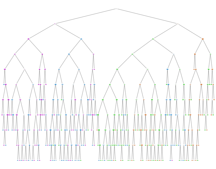
Visualizing the decision tree

from sklearn import tree
fig = plt.figure(figsize=(25,20))
_ = tree.plot_tree(Deci_Tree_best_model, 
                   feature_names=feature_label,  
                   class_names=target_label,
                   filled=True)
plt.savefig('Decision Tree Visualization.png', dpi = 300)
plt.show()

png

Visualizing the decision boundary.

As the no. of dimensions is 10, reducing the no of dimensions to 2 using PCA to visualize a 2D plot of the boundaries

# visualizing the decision regions

from mlxtend.plotting import plot_decision_regions
from sklearn.decomposition import PCA

a = X_train.to_numpy() #changing df to numpy
b = y_train.to_numpy()

pca = PCA(n_components = 2)
a2 = pca.fit_transform(a)

Deci_Tree_best_model.fit(a2, b)

plot_decision_regions(a2, b, clf=Deci_Tree_best_model, legend=2)

# Adding axes annotations
plt.xlabel('ram')
plt.ylabel('battery_power')
plt.title('Decision Tree Boundaries')
plt.savefig('Decision Tree Boundaries (Using PCA).png', dpi = 300)
plt.show()

png

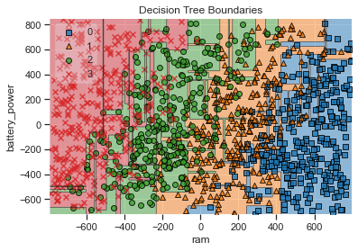
The decision tree model does a better job of demarking the clustered boundaries when compared to the K Means model, hence the improved accuracy score

Model 4: Random Forest

# Model building

from sklearn.ensemble import RandomForestClassifier
RFmodel = RandomForestClassifier()  # Hyperparameters tuning

parameters = {'max_depth':[5,10,15,20,30],
              'random_state': [0,1,2,3,4],
              'n_estimators':[10,30,50,70,100],
              'criterion': ['entropy', 'ginni']
             }  

grid = GridSearchCV(RFmodel,parameters,cv=5,verbose=1) 
grid.fit(X_train,y_train)

Fitting 5 folds for each of 250 candidates, totalling 1250 fits

GridSearchCV(cv=5, estimator=RandomForestClassifier(),
             param_grid={'criterion': ['entropy', 'ginni'],
                         'max_depth': [5, 10, 15, 20, 30],
                         'n_estimators': [10, 30, 50, 70, 100],
                         'random_state': [0, 1, 2, 3, 4]},
             verbose=1)

# Printing the best parameters

print(grid.best_params_)
print(grid.best_estimator_)

{'criterion': 'entropy', 'max_depth': 20, 'n_estimators': 100, 'random_state': 2}
RandomForestClassifier(criterion='entropy', max_depth=20, random_state=2)

# Building the best fit model using the parameters from the grid search

RFBmodel  = RandomForestClassifier(random_state=2, max_depth= 20 , n_estimators=50) 
RFBmodel.fit(X_train, y_train)

RandomForestClassifier(max_depth=20, n_estimators=50, random_state=2)

# Training and testing the model and checking accuracy scores

RFBtrain_predict  = RFBmodel.predict(X_train)
RFBtest_predict   = RFBmodel.predict(X_test)
print(accuracy_score(y_train ,RFBtrain_predict))
RFscore = accuracy_score(y_test , RFBtest_predict)
RFscore

0

896969696969697

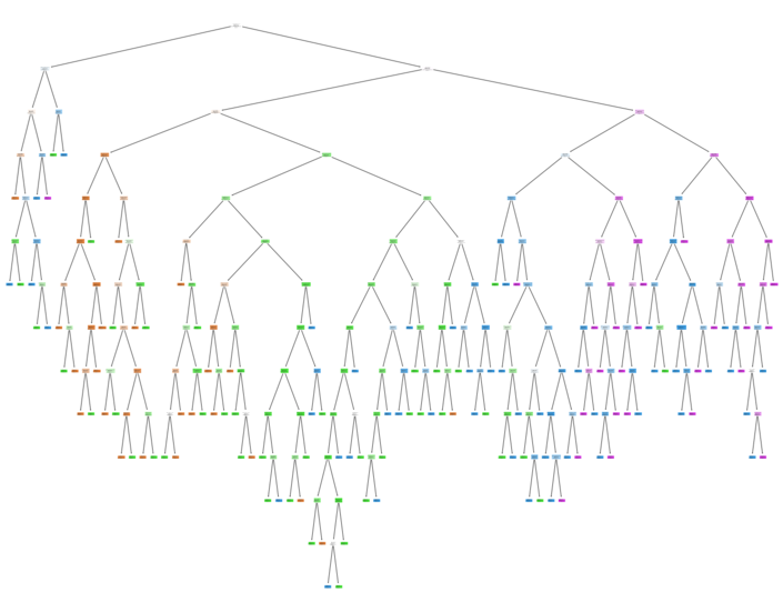
# Visualizing the tree

fig = plt.figure(figsize=(25,20))
_ = tree.plot_tree(RFBmodel.estimators_[0], 
                   feature_names=feature_label,  
                   class_names=target_label,
                   filled=True)
plt.savefig('Random Forest Visualization.png', dpi = 300)
plt.show()

png

Pickling The Model (Save and Load The Model)

with open('rf_pickle', 'wb') as f:
    pickle.dump(RFBmodel, f)

with open('rf_pickle', 'rb') as f:
    model_rf = pickle.load(f)

model_rf.predict(X_test) #testing the model. reason: to make sure the pickle output showing the same as the current model

array([0, 2, 3, 2, 1, 3, 3, 1, 2, 2, 3, 3, 2, 1, 0, 3, 2, 0, 3, 3, 0, 2,
       2, 1, 3, 3, 1, 0, 1, 3, 3, 1, 3, 3, 1, 1, 3, 1, 3, 3, 2, 2, 2, 3,
       1, 2, 2, 0, 3, 0, 1, 2, 0, 3, 2, 0, 1, 3, 2, 1, 0, 2, 2, 1, 0, 2,
       0, 2, 0, 0, 1, 1, 3, 1, 2, 0, 2, 1, 1, 3, 2, 1, 1, 2, 3, 1, 2, 0,
       0, 0, 0, 3, 3, 0, 3, 1, 3, 2, 3, 1, 0, 2, 2, 0, 0, 3, 3, 2, 1, 0,
       2, 1, 1, 0, 0, 0, 2, 3, 3, 2, 0, 0, 1, 0, 3, 2, 0, 0, 0, 2, 3, 1,
       2, 0, 1, 0, 2, 1, 0, 2, 1, 1, 3, 2, 2, 2, 3, 0, 3, 1, 2, 1, 3, 1,
       2, 0, 0, 0, 3, 3, 2, 2, 2, 0, 2, 2, 1, 0, 1, 2, 3, 2, 0, 3, 3, 2,
       1, 0, 1, 2, 1, 0, 2, 2, 1, 3, 3, 0, 2, 3, 3, 0, 1, 1, 2, 1, 3, 2,
       3, 0, 2, 2, 0, 3, 1, 1, 1, 3, 2, 2, 2, 1, 3, 2, 2, 3, 3, 1, 2, 0,
       1, 0, 3, 3, 3, 2, 0, 1, 3, 1, 3, 0, 3, 2, 0, 0, 2, 1, 1, 2, 0, 2,
       0, 1, 3, 3, 2, 0, 1, 1, 0, 0, 3, 0, 3, 2, 3, 0, 1, 1, 1, 1, 3, 1,
       0, 1, 0, 1, 1, 3, 1, 1, 2, 3, 3, 1, 2, 2, 2, 2, 1, 1, 1, 2, 1, 2,
       0, 3, 0, 3, 2, 1, 1, 3, 0, 2, 3, 0, 0, 0, 1, 2, 1, 2, 2, 3, 1, 1,
       1, 1, 0, 0, 1, 1, 2, 2, 1, 0, 2, 0, 2, 3, 3, 0, 2, 3, 0, 2, 2, 2,
       1, 0, 1, 2, 2, 0, 1, 0, 1, 0, 0, 2, 3, 3, 1, 2, 2, 0, 0, 2, 3, 1,
       2, 2, 3, 2, 3, 3, 1, 0, 0, 3, 0, 3, 0, 0, 0, 3, 1, 3, 3, 2, 2, 1,
       1, 3, 0, 1, 0, 1, 1, 3, 0, 1, 1, 3, 0, 0, 2, 0, 1, 1, 2, 3, 2, 3,
       2, 2, 3, 0, 3, 3, 0, 3, 0, 0, 0, 3, 0, 0, 1, 0, 1, 0, 2, 2, 1, 0,
       2, 3, 2, 2, 3, 2, 3, 1, 3, 3, 1, 2, 2, 3, 1, 3, 3, 0, 3, 2, 0, 1,
       0, 2, 3, 0, 0, 0, 1, 0, 0, 0, 3, 1, 0, 1, 1, 2, 0, 3, 1, 1, 0, 2,
       3, 3, 0, 0, 1, 3, 2, 3, 2, 1, 1, 3, 0, 3, 1, 3, 2, 0, 2, 0, 1, 1,
       1, 3, 1, 3, 3, 1, 3, 2, 3, 3, 2, 1, 3, 2, 2, 3, 0, 1, 1, 0, 0, 2,
       2, 1, 1, 1, 3, 1, 0, 2, 3, 2, 2, 1, 1, 0, 1, 1, 0, 0, 1, 3, 2, 2,
       3, 1, 0, 1, 0, 0, 0, 0, 3, 1, 3, 3, 1, 0, 0, 0, 3, 2, 3, 0, 2, 1,
       2, 3, 2, 0, 1, 3, 2, 2, 3, 3, 3, 1, 3, 2, 2, 2, 1, 2, 0, 0, 0, 0,
       0, 3, 2, 0, 0, 2, 1, 0, 0, 0, 1, 3, 3, 0, 2, 3, 1, 0, 1, 3, 1, 2,
       2, 2, 0, 2, 3, 3, 2, 2, 1, 3, 2, 0, 2, 1, 3, 2, 1, 3, 2, 0, 2, 2,
       2, 3, 1, 1, 0, 3, 1, 3, 2, 1, 0, 2, 1, 2, 3, 0, 3, 0, 3, 0, 0, 0,
       1, 1, 1, 2, 2, 1, 0, 3, 0, 2, 2, 3, 2, 0, 2, 1, 1, 3, 2, 0, 1, 0],
      dtype=int64)

Model 5: XG Boost

#! pip install xgboost
# import XGBoost
import xgboost as xgb

# Model building and using gridsearch to get the optimal parameters 

from xgboost import XGBClassifier

params = {
            'objective':'binary:logistic',
            'max_depth': 4,
            'learning_rate': 1.0,
            'n_estimators':100
        }         
      
        
# instantiate the classifier 
xgb_clf = XGBClassifier(**params)


# fit the classifier to the training data
xgb_clf.fit(X_train, y_train)

[13:42:50] WARNING: C:/Users/Administrator/workspace/xgboost-win64_release_1.4.0/src/learner.cc:1095: Starting in XGBoost 1.3.0, the default evaluation metric used with the objective 'multi:softprob' was changed from 'merror' to 'mlogloss'. Explicitly set eval_metric if you'd like to restore the old behavior.





XGBClassifier(base_score=0.5, booster='gbtree', colsample_bylevel=1,
              colsample_bynode=1, colsample_bytree=1, gamma=0, gpu_id=-1,
              importance_type='gain', interaction_constraints='',
              learning_rate=1.0, max_delta_step=0, max_depth=4,
              min_child_weight=1, missing=nan, monotone_constraints='()',
              n_estimators=100, n_jobs=4, num_parallel_tree=1,
              objective='multi:softprob', random_state=0, reg_alpha=0,
              reg_lambda=1, scale_pos_weight=None, subsample=1,
              tree_method='exact', validate_parameters=1, verbosity=None)

# Prediction using the best fit model and checking accuracy scores 

y_pred = xgb_clf.predict(X_test)
XGBscore = accuracy_score(y_test, y_pred)
XGBscore

0.9303030303030303

Pickling The Model (Save and Load The Model)

with open('xgb_pickle', 'wb') as f:
    pickle.dump(xgb_clf, f)

with open('xgb_pickle', 'rb') as f:
    model_xgb = pickle.load(f)

model_xgb.predict(X_test) #testing the model. reason: to make sure the pickle output showing the same as the current model

array([0, 2, 3, 2, 1, 3, 3, 1, 2, 2, 3, 3, 2, 1, 0, 3, 2, 0, 2, 3, 0, 2,
       2, 1, 3, 3, 1, 0, 1, 3, 3, 1, 3, 3, 1, 1, 3, 1, 3, 3, 2, 2, 2, 3,
       2, 2, 2, 0, 3, 0, 0, 2, 0, 3, 2, 0, 1, 3, 2, 0, 0, 2, 2, 1, 0, 2,
       0, 2, 0, 0, 1, 1, 3, 1, 1, 0, 2, 1, 2, 3, 2, 1, 1, 2, 3, 1, 2, 0,
       0, 0, 0, 3, 3, 0, 3, 1, 3, 2, 3, 1, 0, 2, 2, 0, 0, 3, 2, 2, 1, 0,
       2, 1, 1, 1, 0, 0, 2, 3, 3, 2, 0, 0, 1, 0, 3, 2, 0, 0, 0, 2, 3, 1,
       2, 0, 1, 0, 2, 1, 0, 2, 1, 1, 3, 2, 3, 2, 3, 0, 3, 1, 2, 1, 2, 1,
       2, 0, 0, 1, 3, 3, 2, 2, 2, 0, 2, 2, 1, 0, 1, 2, 3, 2, 0, 3, 3, 2,
       1, 0, 1, 2, 1, 0, 2, 2, 0, 3, 2, 0, 2, 3, 3, 0, 1, 2, 2, 2, 3, 1,
       3, 0, 2, 2, 0, 3, 1, 1, 1, 3, 1, 2, 2, 1, 3, 2, 2, 3, 3, 1, 2, 0,
       1, 0, 3, 3, 3, 2, 0, 1, 3, 1, 3, 0, 3, 2, 0, 0, 2, 1, 0, 2, 0, 2,
       0, 1, 3, 3, 1, 0, 2, 1, 0, 0, 3, 0, 3, 2, 3, 1, 2, 1, 1, 1, 3, 1,
       0, 1, 0, 1, 1, 3, 1, 1, 2, 3, 3, 1, 3, 3, 2, 1, 2, 1, 1, 2, 1, 2,
       0, 3, 0, 3, 3, 1, 1, 3, 0, 2, 3, 0, 0, 0, 2, 1, 1, 2, 3, 2, 1, 1,
       1, 1, 0, 0, 1, 1, 2, 2, 1, 0, 2, 0, 2, 3, 3, 0, 2, 3, 0, 2, 2, 2,
       1, 0, 1, 2, 2, 0, 1, 0, 1, 0, 0, 2, 3, 3, 1, 2, 2, 0, 0, 1, 3, 1,
       2, 2, 3, 2, 3, 3, 1, 0, 0, 3, 0, 3, 0, 0, 0, 3, 1, 3, 3, 2, 1, 1,
       1, 3, 0, 1, 0, 1, 1, 3, 0, 1, 1, 3, 0, 0, 2, 0, 2, 1, 2, 3, 2, 3,
       1, 2, 3, 0, 3, 3, 0, 3, 0, 0, 0, 3, 0, 0, 1, 0, 1, 0, 2, 2, 1, 0,
       3, 3, 2, 2, 3, 2, 3, 1, 3, 3, 1, 2, 2, 3, 1, 3, 3, 0, 3, 1, 0, 1,
       0, 2, 3, 0, 0, 0, 1, 1, 0, 0, 3, 1, 0, 1, 1, 3, 1, 3, 1, 1, 0, 1,
       3, 3, 0, 0, 1, 3, 2, 3, 3, 1, 1, 2, 0, 3, 1, 3, 2, 0, 2, 0, 1, 1,
       2, 3, 1, 3, 3, 1, 3, 2, 3, 3, 2, 1, 3, 2, 2, 3, 0, 1, 1, 0, 0, 2,
       2, 1, 1, 1, 3, 0, 0, 2, 3, 2, 2, 1, 1, 0, 1, 1, 0, 0, 1, 3, 2, 2,
       3, 1, 0, 1, 0, 0, 0, 0, 3, 1, 3, 3, 2, 0, 0, 1, 3, 2, 3, 0, 2, 1,
       2, 3, 2, 0, 1, 3, 2, 2, 3, 3, 3, 1, 3, 2, 2, 2, 1, 2, 0, 0, 0, 1,
       0, 3, 2, 0, 0, 2, 1, 0, 0, 0, 1, 3, 3, 0, 2, 3, 1, 0, 1, 3, 1, 2,
       2, 2, 0, 3, 3, 3, 2, 2, 2, 2, 2, 0, 2, 1, 3, 2, 1, 3, 2, 0, 2, 2,
       2, 3, 1, 1, 0, 3, 1, 3, 2, 1, 0, 2, 1, 2, 3, 0, 3, 0, 3, 0, 0, 0,
       1, 0, 1, 2, 2, 1, 0, 3, 0, 2, 2, 3, 2, 0, 2, 1, 1, 3, 2, 0, 1, 0],
      dtype=int64)

Model 6: SVM Classification

from sklearn.svm import SVC
from sklearn.metrics import classification_report
from mlxtend.plotting import plot_decision_regions
from sklearn.svm import SVC

# Building the best fit model using the gridsearch methodology

param_grid = {'C': [0.1, 1, 10, 100, 1000], 
              'gamma': [1, 0.1, 0.01, 0.001, 0.0001],
              'kernel': ['rbf', 'poly']} 
  
grid = GridSearchCV(SVC(), param_grid, refit = True, verbose = 3)
  
# fitting the model for grid search
grid.fit(X_train, y_train)

Fitting 5 folds for each of 50 candidates, totalling 250 fits
[CV 1/5] END ........C=0.1, gamma=1, kernel=rbf;, score=0.250 total time=   0.2s
[CV 2/5] END ........C=0.1, gamma=1, kernel=rbf;, score=0.250 total time=   0.2s
[CV 3/5] END ........C=0.1, gamma=1, kernel=rbf;, score=0.250 total time=   0.2s
[CV 4/5] END ........C=0.1, gamma=1, kernel=rbf;, score=0.250 total time=   0.2s
[CV 5/5] END ........C=0.1, gamma=1, kernel=rbf;, score=0.250 total time=   0.2s
[CV 1/5] END .......C=0.1, gamma=1, kernel=poly;, score=0.970 total time=   0.0s
[CV 2/5] END .......C=0.1, gamma=1, kernel=poly;, score=0.948 total time=   0.0s
[CV 3/5] END .......C=0.1, gamma=1, kernel=poly;, score=0.944 total time=   0.0s
[CV 4/5] END .......C=0.1, gamma=1, kernel=poly;, score=0.944 total time=   0.0s
[CV 5/5] END .......C=0.1, gamma=1, kernel=poly;, score=0.929 total time=   0.0s
[CV 1/5] END ......C=0.1, gamma=0.1, kernel=rbf;, score=0.313 total time=   0.2s
[CV 2/5] END ......C=0.1, gamma=0.1, kernel=rbf;, score=0.306 total time=   0.2s
[CV 3/5] END ......C=0.1, gamma=0.1, kernel=rbf;, score=0.313 total time=   0.2s
[CV 4/5] END ......C=0.1, gamma=0.1, kernel=rbf;, score=0.299 total time=   0.2s
[CV 5/5] END ......C=0.1, gamma=0.1, kernel=rbf;, score=0.295 total time=   0.2s
[CV 1/5] END .....C=0.1, gamma=0.1, kernel=poly;, score=0.970 total time=   0.1s
[CV 2/5] END .....C=0.1, gamma=0.1, kernel=poly;, score=0.948 total time=   0.0s
[CV 3/5] END .....C=0.1, gamma=0.1, kernel=poly;, score=0.944 total time=   0.0s
[CV 4/5] END .....C=0.1, gamma=0.1, kernel=poly;, score=0.944 total time=   0.0s
[CV 5/5] END .....C=0.1, gamma=0.1, kernel=poly;, score=0.929 total time=   0.0s
[CV 1/5] END .....C=0.1, gamma=0.01, kernel=rbf;, score=0.500 total time=   0.2s
[CV 2/5] END .....C=0.1, gamma=0.01, kernel=rbf;, score=0.500 total time=   0.2s
[CV 3/5] END .....C=0.1, gamma=0.01, kernel=rbf;, score=0.496 total time=   0.2s
[CV 4/5] END .....C=0.1, gamma=0.01, kernel=rbf;, score=0.496 total time=   0.2s
[CV 5/5] END .....C=0.1, gamma=0.01, kernel=rbf;, score=0.683 total time=   0.2s
[CV 1/5] END ....C=0.1, gamma=0.01, kernel=poly;, score=0.970 total time=   0.0s
[CV 2/5] END ....C=0.1, gamma=0.01, kernel=poly;, score=0.948 total time=   0.0s
[CV 3/5] END ....C=0.1, gamma=0.01, kernel=poly;, score=0.944 total time=   0.0s
[CV 4/5] END ....C=0.1, gamma=0.01, kernel=poly;, score=0.944 total time=   0.0s
[CV 5/5] END ....C=0.1, gamma=0.01, kernel=poly;, score=0.929 total time=   0.0s
[CV 1/5] END ....C=0.1, gamma=0.001, kernel=rbf;, score=0.265 total time=   0.1s
[CV 2/5] END ....C=0.1, gamma=0.001, kernel=rbf;, score=0.257 total time=   0.1s
[CV 3/5] END ....C=0.1, gamma=0.001, kernel=rbf;, score=0.261 total time=   0.2s
[CV 4/5] END ....C=0.1, gamma=0.001, kernel=rbf;, score=0.265 total time=   0.1s
[CV 5/5] END ....C=0.1, gamma=0.001, kernel=rbf;, score=0.272 total time=   0.1s
[CV 1/5] END ...C=0.1, gamma=0.001, kernel=poly;, score=0.970 total time=   0.1s
[CV 2/5] END ...C=0.1, gamma=0.001, kernel=poly;, score=0.948 total time=   0.0s
[CV 3/5] END ...C=0.1, gamma=0.001, kernel=poly;, score=0.944 total time=   0.0s
[CV 4/5] END ...C=0.1, gamma=0.001, kernel=poly;, score=0.944 total time=   0.0s
[CV 5/5] END ...C=0.1, gamma=0.001, kernel=poly;, score=0.929 total time=   0.0s
[CV 1/5] END ...C=0.1, gamma=0.0001, kernel=rbf;, score=0.698 total time=   0.1s
[CV 2/5] END ...C=0.1, gamma=0.0001, kernel=rbf;, score=0.646 total time=   0.1s
[CV 3/5] END ...C=0.1, gamma=0.0001, kernel=rbf;, score=0.694 total time=   0.1s
[CV 4/5] END ...C=0.1, gamma=0.0001, kernel=rbf;, score=0.552 total time=   0.1s
[CV 5/5] END ...C=0.1, gamma=0.0001, kernel=rbf;, score=0.754 total time=   0.1s
[CV 1/5] END ..C=0.1, gamma=0.0001, kernel=poly;, score=0.970 total time=   0.0s
[CV 2/5] END ..C=0.1, gamma=0.0001, kernel=poly;, score=0.948 total time=   0.0s
[CV 3/5] END ..C=0.1, gamma=0.0001, kernel=poly;, score=0.944 total time=   0.0s
[CV 4/5] END ..C=0.1, gamma=0.0001, kernel=poly;, score=0.944 total time=   0.0s
[CV 5/5] END ..C=0.1, gamma=0.0001, kernel=poly;, score=0.929 total time=   0.0s
[CV 1/5] END ..........C=1, gamma=1, kernel=rbf;, score=0.250 total time=   0.1s
[CV 2/5] END ..........C=1, gamma=1, kernel=rbf;, score=0.250 total time=   0.2s
[CV 3/5] END ..........C=1, gamma=1, kernel=rbf;, score=0.250 total time=   0.1s
[CV 4/5] END ..........C=1, gamma=1, kernel=rbf;, score=0.250 total time=   0.2s
[CV 5/5] END ..........C=1, gamma=1, kernel=rbf;, score=0.250 total time=   0.2s
[CV 1/5] END .........C=1, gamma=1, kernel=poly;, score=0.970 total time=   0.0s
[CV 2/5] END .........C=1, gamma=1, kernel=poly;, score=0.948 total time=   0.0s
[CV 3/5] END .........C=1, gamma=1, kernel=poly;, score=0.944 total time=   0.0s
[CV 4/5] END .........C=1, gamma=1, kernel=poly;, score=0.944 total time=   0.0s
[CV 5/5] END .........C=1, gamma=1, kernel=poly;, score=0.929 total time=   0.0s
[CV 1/5] END ........C=1, gamma=0.1, kernel=rbf;, score=0.295 total time=   0.2s
[CV 2/5] END ........C=1, gamma=0.1, kernel=rbf;, score=0.284 total time=   0.2s
[CV 3/5] END ........C=1, gamma=0.1, kernel=rbf;, score=0.295 total time=   0.1s
[CV 4/5] END ........C=1, gamma=0.1, kernel=rbf;, score=0.291 total time=   0.2s
[CV 5/5] END ........C=1, gamma=0.1, kernel=rbf;, score=0.295 total time=   0.1s
[CV 1/5] END .......C=1, gamma=0.1, kernel=poly;, score=0.970 total time=   0.1s
[CV 2/5] END .......C=1, gamma=0.1, kernel=poly;, score=0.948 total time=   0.0s
[CV 3/5] END .......C=1, gamma=0.1, kernel=poly;, score=0.944 total time=   0.0s
[CV 4/5] END .......C=1, gamma=0.1, kernel=poly;, score=0.944 total time=   0.0s
[CV 5/5] END .......C=1, gamma=0.1, kernel=poly;, score=0.929 total time=   0.0s
[CV 1/5] END .......C=1, gamma=0.01, kernel=rbf;, score=0.250 total time=   0.2s
[CV 2/5] END .......C=1, gamma=0.01, kernel=rbf;, score=0.254 total time=   0.2s
[CV 3/5] END .......C=1, gamma=0.01, kernel=rbf;, score=0.250 total time=   0.2s
[CV 4/5] END .......C=1, gamma=0.01, kernel=rbf;, score=0.250 total time=   0.2s
[CV 5/5] END .......C=1, gamma=0.01, kernel=rbf;, score=0.254 total time=   0.2s
[CV 1/5] END ......C=1, gamma=0.01, kernel=poly;, score=0.970 total time=   0.0s
[CV 2/5] END ......C=1, gamma=0.01, kernel=poly;, score=0.948 total time=   0.0s
[CV 3/5] END ......C=1, gamma=0.01, kernel=poly;, score=0.944 total time=   0.0s
[CV 4/5] END ......C=1, gamma=0.01, kernel=poly;, score=0.944 total time=   0.0s
[CV 5/5] END ......C=1, gamma=0.01, kernel=poly;, score=0.929 total time=   0.0s
[CV 1/5] END ......C=1, gamma=0.001, kernel=rbf;, score=0.313 total time=   0.2s
[CV 2/5] END ......C=1, gamma=0.001, kernel=rbf;, score=0.310 total time=   0.2s
[CV 3/5] END ......C=1, gamma=0.001, kernel=rbf;, score=0.310 total time=   0.1s
[CV 4/5] END ......C=1, gamma=0.001, kernel=rbf;, score=0.332 total time=   0.2s
[CV 5/5] END ......C=1, gamma=0.001, kernel=rbf;, score=0.306 total time=   0.1s
[CV 1/5] END .....C=1, gamma=0.001, kernel=poly;, score=0.970 total time=   0.1s
[CV 2/5] END .....C=1, gamma=0.001, kernel=poly;, score=0.948 total time=   0.0s
[CV 3/5] END .....C=1, gamma=0.001, kernel=poly;, score=0.944 total time=   0.0s
[CV 4/5] END .....C=1, gamma=0.001, kernel=poly;, score=0.944 total time=   0.0s
[CV 5/5] END .....C=1, gamma=0.001, kernel=poly;, score=0.929 total time=   0.0s
[CV 1/5] END .....C=1, gamma=0.0001, kernel=rbf;, score=0.899 total time=   0.1s
[CV 2/5] END .....C=1, gamma=0.0001, kernel=rbf;, score=0.896 total time=   0.1s
[CV 3/5] END .....C=1, gamma=0.0001, kernel=rbf;, score=0.892 total time=   0.1s
[CV 4/5] END .....C=1, gamma=0.0001, kernel=rbf;, score=0.825 total time=   0.2s
[CV 5/5] END .....C=1, gamma=0.0001, kernel=rbf;, score=0.858 total time=   0.1s
[CV 1/5] END ....C=1, gamma=0.0001, kernel=poly;, score=0.970 total time=   0.0s
[CV 2/5] END ....C=1, gamma=0.0001, kernel=poly;, score=0.948 total time=   0.0s
[CV 3/5] END ....C=1, gamma=0.0001, kernel=poly;, score=0.944 total time=   0.0s
[CV 4/5] END ....C=1, gamma=0.0001, kernel=poly;, score=0.944 total time=   0.0s
[CV 5/5] END ....C=1, gamma=0.0001, kernel=poly;, score=0.929 total time=   0.0s
[CV 1/5] END .........C=10, gamma=1, kernel=rbf;, score=0.250 total time=   0.2s
[CV 2/5] END .........C=10, gamma=1, kernel=rbf;, score=0.250 total time=   0.2s
[CV 3/5] END .........C=10, gamma=1, kernel=rbf;, score=0.250 total time=   0.2s
[CV 4/5] END .........C=10, gamma=1, kernel=rbf;, score=0.250 total time=   0.2s
[CV 5/5] END .........C=10, gamma=1, kernel=rbf;, score=0.250 total time=   0.2s
[CV 1/5] END ........C=10, gamma=1, kernel=poly;, score=0.970 total time=   0.0s
[CV 2/5] END ........C=10, gamma=1, kernel=poly;, score=0.948 total time=   0.0s
[CV 3/5] END ........C=10, gamma=1, kernel=poly;, score=0.944 total time=   0.0s
[CV 4/5] END ........C=10, gamma=1, kernel=poly;, score=0.944 total time=   0.0s
[CV 5/5] END ........C=10, gamma=1, kernel=poly;, score=0.929 total time=   0.0s
[CV 1/5] END .......C=10, gamma=0.1, kernel=rbf;, score=0.295 total time=   0.2s
[CV 2/5] END .......C=10, gamma=0.1, kernel=rbf;, score=0.284 total time=   0.2s
[CV 3/5] END .......C=10, gamma=0.1, kernel=rbf;, score=0.295 total time=   0.2s
[CV 4/5] END .......C=10, gamma=0.1, kernel=rbf;, score=0.291 total time=   0.2s
[CV 5/5] END .......C=10, gamma=0.1, kernel=rbf;, score=0.295 total time=   0.2s
[CV 1/5] END ......C=10, gamma=0.1, kernel=poly;, score=0.970 total time=   0.1s
[CV 2/5] END ......C=10, gamma=0.1, kernel=poly;, score=0.948 total time=   0.0s
[CV 3/5] END ......C=10, gamma=0.1, kernel=poly;, score=0.944 total time=   0.0s
[CV 4/5] END ......C=10, gamma=0.1, kernel=poly;, score=0.944 total time=   0.0s
[CV 5/5] END ......C=10, gamma=0.1, kernel=poly;, score=0.929 total time=   0.0s
[CV 1/5] END ......C=10, gamma=0.01, kernel=rbf;, score=0.250 total time=   0.2s
[CV 2/5] END ......C=10, gamma=0.01, kernel=rbf;, score=0.254 total time=   0.2s
[CV 3/5] END ......C=10, gamma=0.01, kernel=rbf;, score=0.250 total time=   0.2s
[CV 4/5] END ......C=10, gamma=0.01, kernel=rbf;, score=0.250 total time=   0.1s
[CV 5/5] END ......C=10, gamma=0.01, kernel=rbf;, score=0.254 total time=   0.1s
[CV 1/5] END .....C=10, gamma=0.01, kernel=poly;, score=0.970 total time=   0.0s
[CV 2/5] END .....C=10, gamma=0.01, kernel=poly;, score=0.948 total time=   0.0s
[CV 3/5] END .....C=10, gamma=0.01, kernel=poly;, score=0.944 total time=   0.0s
[CV 4/5] END .....C=10, gamma=0.01, kernel=poly;, score=0.944 total time=   0.0s
[CV 5/5] END .....C=10, gamma=0.01, kernel=poly;, score=0.929 total time=   0.0s
[CV 1/5] END .....C=10, gamma=0.001, kernel=rbf;, score=0.317 total time=   0.2s
[CV 2/5] END .....C=10, gamma=0.001, kernel=rbf;, score=0.317 total time=   0.2s
[CV 3/5] END .....C=10, gamma=0.001, kernel=rbf;, score=0.321 total time=   0.1s
[CV 4/5] END .....C=10, gamma=0.001, kernel=rbf;, score=0.343 total time=   0.1s
[CV 5/5] END .....C=10, gamma=0.001, kernel=rbf;, score=0.317 total time=   0.1s
[CV 1/5] END ....C=10, gamma=0.001, kernel=poly;, score=0.970 total time=   0.1s
[CV 2/5] END ....C=10, gamma=0.001, kernel=poly;, score=0.948 total time=   0.0s
[CV 3/5] END ....C=10, gamma=0.001, kernel=poly;, score=0.944 total time=   0.0s
[CV 4/5] END ....C=10, gamma=0.001, kernel=poly;, score=0.944 total time=   0.0s
[CV 5/5] END ....C=10, gamma=0.001, kernel=poly;, score=0.929 total time=   0.0s
[CV 1/5] END ....C=10, gamma=0.0001, kernel=rbf;, score=0.899 total time=   0.1s
[CV 2/5] END ....C=10, gamma=0.0001, kernel=rbf;, score=0.899 total time=   0.1s
[CV 3/5] END ....C=10, gamma=0.0001, kernel=rbf;, score=0.896 total time=   0.1s
[CV 4/5] END ....C=10, gamma=0.0001, kernel=rbf;, score=0.828 total time=   0.1s
[CV 5/5] END ....C=10, gamma=0.0001, kernel=rbf;, score=0.862 total time=   0.1s
[CV 1/5] END ...C=10, gamma=0.0001, kernel=poly;, score=0.970 total time=   0.0s
[CV 2/5] END ...C=10, gamma=0.0001, kernel=poly;, score=0.948 total time=   0.0s
[CV 3/5] END ...C=10, gamma=0.0001, kernel=poly;, score=0.944 total time=   0.0s
[CV 4/5] END ...C=10, gamma=0.0001, kernel=poly;, score=0.944 total time=   0.0s
[CV 5/5] END ...C=10, gamma=0.0001, kernel=poly;, score=0.929 total time=   0.0s
[CV 1/5] END ........C=100, gamma=1, kernel=rbf;, score=0.250 total time=   0.2s
[CV 2/5] END ........C=100, gamma=1, kernel=rbf;, score=0.250 total time=   0.2s
[CV 3/5] END ........C=100, gamma=1, kernel=rbf;, score=0.250 total time=   0.2s
[CV 4/5] END ........C=100, gamma=1, kernel=rbf;, score=0.250 total time=   0.2s
[CV 5/5] END ........C=100, gamma=1, kernel=rbf;, score=0.250 total time=   0.2s
[CV 1/5] END .......C=100, gamma=1, kernel=poly;, score=0.970 total time=   0.0s
[CV 2/5] END .......C=100, gamma=1, kernel=poly;, score=0.948 total time=   0.0s
[CV 3/5] END .......C=100, gamma=1, kernel=poly;, score=0.944 total time=   0.0s
[CV 4/5] END .......C=100, gamma=1, kernel=poly;, score=0.944 total time=   0.0s
[CV 5/5] END .......C=100, gamma=1, kernel=poly;, score=0.929 total time=   0.0s
[CV 1/5] END ......C=100, gamma=0.1, kernel=rbf;, score=0.295 total time=   0.2s
[CV 2/5] END ......C=100, gamma=0.1, kernel=rbf;, score=0.284 total time=   0.2s
[CV 3/5] END ......C=100, gamma=0.1, kernel=rbf;, score=0.295 total time=   0.1s
[CV 4/5] END ......C=100, gamma=0.1, kernel=rbf;, score=0.291 total time=   0.2s
[CV 5/5] END ......C=100, gamma=0.1, kernel=rbf;, score=0.295 total time=   0.2s
[CV 1/5] END .....C=100, gamma=0.1, kernel=poly;, score=0.970 total time=   0.1s
[CV 2/5] END .....C=100, gamma=0.1, kernel=poly;, score=0.948 total time=   0.0s
[CV 3/5] END .....C=100, gamma=0.1, kernel=poly;, score=0.944 total time=   0.0s
[CV 4/5] END .....C=100, gamma=0.1, kernel=poly;, score=0.944 total time=   0.0s
[CV 5/5] END .....C=100, gamma=0.1, kernel=poly;, score=0.929 total time=   0.0s
[CV 1/5] END .....C=100, gamma=0.01, kernel=rbf;, score=0.250 total time=   0.2s
[CV 2/5] END .....C=100, gamma=0.01, kernel=rbf;, score=0.254 total time=   0.1s
[CV 3/5] END .....C=100, gamma=0.01, kernel=rbf;, score=0.250 total time=   0.2s
[CV 4/5] END .....C=100, gamma=0.01, kernel=rbf;, score=0.250 total time=   0.2s
[CV 5/5] END .....C=100, gamma=0.01, kernel=rbf;, score=0.254 total time=   0.1s
[CV 1/5] END ....C=100, gamma=0.01, kernel=poly;, score=0.970 total time=   0.0s
[CV 2/5] END ....C=100, gamma=0.01, kernel=poly;, score=0.948 total time=   0.0s
[CV 3/5] END ....C=100, gamma=0.01, kernel=poly;, score=0.944 total time=   0.0s
[CV 4/5] END ....C=100, gamma=0.01, kernel=poly;, score=0.944 total time=   0.0s
[CV 5/5] END ....C=100, gamma=0.01, kernel=poly;, score=0.929 total time=   0.0s
[CV 1/5] END ....C=100, gamma=0.001, kernel=rbf;, score=0.317 total time=   0.2s
[CV 2/5] END ....C=100, gamma=0.001, kernel=rbf;, score=0.317 total time=   0.1s
[CV 3/5] END ....C=100, gamma=0.001, kernel=rbf;, score=0.321 total time=   0.2s
[CV 4/5] END ....C=100, gamma=0.001, kernel=rbf;, score=0.343 total time=   0.2s
[CV 5/5] END ....C=100, gamma=0.001, kernel=rbf;, score=0.317 total time=   0.1s
[CV 1/5] END ...C=100, gamma=0.001, kernel=poly;, score=0.970 total time=   0.1s
[CV 2/5] END ...C=100, gamma=0.001, kernel=poly;, score=0.948 total time=   0.0s
[CV 3/5] END ...C=100, gamma=0.001, kernel=poly;, score=0.944 total time=   0.0s
[CV 4/5] END ...C=100, gamma=0.001, kernel=poly;, score=0.944 total time=   0.0s
[CV 5/5] END ...C=100, gamma=0.001, kernel=poly;, score=0.929 total time=   0.0s
[CV 1/5] END ...C=100, gamma=0.0001, kernel=rbf;, score=0.899 total time=   0.1s
[CV 2/5] END ...C=100, gamma=0.0001, kernel=rbf;, score=0.899 total time=   0.1s
[CV 3/5] END ...C=100, gamma=0.0001, kernel=rbf;, score=0.896 total time=   0.1s
[CV 4/5] END ...C=100, gamma=0.0001, kernel=rbf;, score=0.828 total time=   0.1s
[CV 5/5] END ...C=100, gamma=0.0001, kernel=rbf;, score=0.862 total time=   0.1s
[CV 1/5] END ..C=100, gamma=0.0001, kernel=poly;, score=0.970 total time=   0.0s
[CV 2/5] END ..C=100, gamma=0.0001, kernel=poly;, score=0.948 total time=   0.0s
[CV 3/5] END ..C=100, gamma=0.0001, kernel=poly;, score=0.944 total time=   0.0s
[CV 4/5] END ..C=100, gamma=0.0001, kernel=poly;, score=0.944 total time=   0.0s
[CV 5/5] END ..C=100, gamma=0.0001, kernel=poly;, score=0.929 total time=   0.0s
[CV 1/5] END .......C=1000, gamma=1, kernel=rbf;, score=0.250 total time=   0.2s
[CV 2/5] END .......C=1000, gamma=1, kernel=rbf;, score=0.250 total time=   0.2s
[CV 3/5] END .......C=1000, gamma=1, kernel=rbf;, score=0.250 total time=   0.2s
[CV 4/5] END .......C=1000, gamma=1, kernel=rbf;, score=0.250 total time=   0.1s
[CV 5/5] END .......C=1000, gamma=1, kernel=rbf;, score=0.250 total time=   0.2s
[CV 1/5] END ......C=1000, gamma=1, kernel=poly;, score=0.970 total time=   0.0s
[CV 2/5] END ......C=1000, gamma=1, kernel=poly;, score=0.948 total time=   0.0s
[CV 3/5] END ......C=1000, gamma=1, kernel=poly;, score=0.944 total time=   0.0s
[CV 4/5] END ......C=1000, gamma=1, kernel=poly;, score=0.944 total time=   0.0s
[CV 5/5] END ......C=1000, gamma=1, kernel=poly;, score=0.929 total time=   0.0s
[CV 1/5] END .....C=1000, gamma=0.1, kernel=rbf;, score=0.295 total time=   0.2s
[CV 2/5] END .....C=1000, gamma=0.1, kernel=rbf;, score=0.284 total time=   0.2s
[CV 3/5] END .....C=1000, gamma=0.1, kernel=rbf;, score=0.295 total time=   0.2s
[CV 4/5] END .....C=1000, gamma=0.1, kernel=rbf;, score=0.291 total time=   0.2s
[CV 5/5] END .....C=1000, gamma=0.1, kernel=rbf;, score=0.295 total time=   0.2s
[CV 1/5] END ....C=1000, gamma=0.1, kernel=poly;, score=0.970 total time=   0.1s
[CV 2/5] END ....C=1000, gamma=0.1, kernel=poly;, score=0.948 total time=   0.0s
[CV 3/5] END ....C=1000, gamma=0.1, kernel=poly;, score=0.944 total time=   0.0s
[CV 4/5] END ....C=1000, gamma=0.1, kernel=poly;, score=0.944 total time=   0.0s
[CV 5/5] END ....C=1000, gamma=0.1, kernel=poly;, score=0.929 total time=   0.0s
[CV 1/5] END ....C=1000, gamma=0.01, kernel=rbf;, score=0.250 total time=   0.2s
[CV 2/5] END ....C=1000, gamma=0.01, kernel=rbf;, score=0.254 total time=   0.2s
[CV 3/5] END ....C=1000, gamma=0.01, kernel=rbf;, score=0.250 total time=   0.2s
[CV 4/5] END ....C=1000, gamma=0.01, kernel=rbf;, score=0.250 total time=   0.2s
[CV 5/5] END ....C=1000, gamma=0.01, kernel=rbf;, score=0.254 total time=   0.2s
[CV 1/5] END ...C=1000, gamma=0.01, kernel=poly;, score=0.970 total time=   0.0s
[CV 2/5] END ...C=1000, gamma=0.01, kernel=poly;, score=0.948 total time=   0.0s
[CV 3/5] END ...C=1000, gamma=0.01, kernel=poly;, score=0.944 total time=   0.0s
[CV 4/5] END ...C=1000, gamma=0.01, kernel=poly;, score=0.944 total time=   0.0s
[CV 5/5] END ...C=1000, gamma=0.01, kernel=poly;, score=0.929 total time=   0.0s
[CV 1/5] END ...C=1000, gamma=0.001, kernel=rbf;, score=0.317 total time=   0.1s
[CV 2/5] END ...C=1000, gamma=0.001, kernel=rbf;, score=0.317 total time=   0.2s
[CV 3/5] END ...C=1000, gamma=0.001, kernel=rbf;, score=0.321 total time=   0.2s
[CV 4/5] END ...C=1000, gamma=0.001, kernel=rbf;, score=0.343 total time=   0.1s
[CV 5/5] END ...C=1000, gamma=0.001, kernel=rbf;, score=0.317 total time=   0.2s
[CV 1/5] END ..C=1000, gamma=0.001, kernel=poly;, score=0.970 total time=   0.1s
[CV 2/5] END ..C=1000, gamma=0.001, kernel=poly;, score=0.948 total time=   0.0s
[CV 3/5] END ..C=1000, gamma=0.001, kernel=poly;, score=0.944 total time=   0.0s
[CV 4/5] END ..C=1000, gamma=0.001, kernel=poly;, score=0.944 total time=   0.0s
[CV 5/5] END ..C=1000, gamma=0.001, kernel=poly;, score=0.929 total time=   0.0s
[CV 1/5] END ..C=1000, gamma=0.0001, kernel=rbf;, score=0.899 total time=   0.1s
[CV 2/5] END ..C=1000, gamma=0.0001, kernel=rbf;, score=0.899 total time=   0.1s
[CV 3/5] END ..C=1000, gamma=0.0001, kernel=rbf;, score=0.896 total time=   0.1s
[CV 4/5] END ..C=1000, gamma=0.0001, kernel=rbf;, score=0.828 total time=   0.1s
[CV 5/5] END ..C=1000, gamma=0.0001, kernel=rbf;, score=0.862 total time=   0.1s
[CV 1/5] END .C=1000, gamma=0.0001, kernel=poly;, score=0.970 total time=   0.0s
[CV 2/5] END .C=1000, gamma=0.0001, kernel=poly;, score=0.948 total time=   0.0s
[CV 3/5] END .C=1000, gamma=0.0001, kernel=poly;, score=0.944 total time=   0.0s
[CV 4/5] END .C=1000, gamma=0.0001, kernel=poly;, score=0.944 total time=   0.0s
[CV 5/5] END .C=1000, gamma=0.0001, kernel=poly;, score=0.929 total time=   0.0s





GridSearchCV(estimator=SVC(),
             param_grid={'C': [0.1, 1, 10, 100, 1000],
                         'gamma': [1, 0.1, 0.01, 0.001, 0.0001],
                         'kernel': ['rbf', 'poly']},
             verbose=3)

# print best parameter after tuning
print(grid.best_params_)
  
# print how our model looks after hyper-parameter tuning
print(grid.best_estimator_)

{'C': 0.1, 'gamma': 1, 'kernel': 'poly'}
SVC(C=0.1, gamma=1, kernel='poly')

# Running the bestfit model and checking for accuracy scores

svc =  SVC(C=0.1, gamma=1, kernel='poly')
svc.fit(X_train, y_train)
svc_predicted = svc.predict(X_test)
svc_conf_matrix = confusion_matrix(y_test, svc_predicted)
svc_acc_score = accuracy_score(y_test, svc_predicted)
print("confussion matrix")
print(svc_conf_matrix)
print("-------------------------------------------")
print("Accuracy of Support Vector Classifier:",svc_acc_score*100,'\n')
print("-------------------------------------------")
print(classification_report(y_test,svc_predicted))

confussion matrix
[[162   3   0   0]
 [  2 158   5   0]
 [  0   2 155   8]
 [  0   0   5 160]]
-------------------------------------------
Accuracy of Support Vector Classifier: 96.21212121212122 

-------------------------------------------
              precision    recall  f1-score   support

           0       0.99      0.98      0.98       165
           1       0.97      0.96      0.96       165
           2       0.94      0.94      0.94       165
           3       0.95      0.97      0.96       165

    accuracy                           0.96       660
   macro avg       0.96      0.96      0.96       660
weighted avg       0.96      0.96      0.96       660

Visualizing the classification boundaries for SVC…but since it is taking a long time to process the code has been commented

#m = X_train.to_numpy() #changing df to numpy
#n = y_train.to_numpy()

#plot_decision_regions(m, n,clf=svc, legend =4) 

# Adding axes annotations
#plt.xlabel('ram')
#plt.ylabel('battery_power')
#plt.title('SVM Boundaries')
#plt.show()

# Training and testing the best fit model from the gridsearch

svc_train_predict  = svc.predict(X_train)
svc_test_predict   = svc.predict(X_test)

# checking the accuracy of the best fit model

print(accuracy_score(y_train ,svc_train_predict))
SVCscore = accuracy_score(y_test ,svc_test_predict)
SVCscore

0

9621212121212122

Pickling The Model (Save and Load The Model)

with open('svc_pickle', 'wb') as f:
    pickle.dump(svc, f)

with open('svc_pickle', 'rb') as f:
    model_svc = pickle.load(f)

model_svc.predict(X_test) #testing the model. reason: to make sure the pickle output showing the same as the current model

array([0, 2, 3, 3, 1, 3, 3, 1, 2, 2, 3, 3, 2, 1, 0, 3, 2, 0, 3, 3, 0, 2,
       2, 1, 3, 3, 1, 0, 1, 3, 3, 1, 3, 3, 1, 1, 3, 1, 3, 3, 2, 2, 2, 3,
       2, 3, 2, 0, 3, 0, 0, 2, 0, 2, 1, 0, 1, 3, 2, 0, 0, 2, 2, 0, 0, 2,
       0, 2, 0, 0, 1, 2, 3, 1, 1, 0, 2, 1, 1, 3, 3, 1, 1, 1, 3, 1, 2, 0,
       0, 0, 0, 3, 3, 0, 3, 1, 3, 2, 3, 1, 0, 2, 2, 0, 0, 3, 2, 2, 1, 0,
       2, 2, 1, 1, 0, 0, 2, 3, 3, 2, 1, 0, 1, 0, 3, 2, 0, 0, 0, 2, 3, 1,
       2, 0, 1, 0, 2, 1, 0, 2, 1, 1, 3, 2, 3, 2, 3, 0, 3, 1, 2, 1, 3, 1,
       2, 0, 0, 1, 3, 3, 2, 2, 2, 0, 2, 2, 1, 0, 1, 2, 3, 2, 0, 3, 3, 2,
       2, 0, 1, 2, 1, 0, 2, 2, 0, 3, 2, 0, 2, 3, 3, 0, 2, 2, 2, 2, 3, 1,
       3, 0, 2, 2, 0, 3, 1, 1, 1, 3, 1, 2, 2, 1, 3, 2, 3, 3, 3, 1, 2, 0,
       1, 0, 3, 3, 3, 2, 0, 1, 3, 1, 3, 0, 3, 2, 0, 0, 2, 1, 0, 3, 0, 2,
       0, 1, 3, 3, 2, 0, 2, 1, 0, 0, 3, 0, 3, 2, 3, 1, 1, 1, 1, 1, 3, 1,
       0, 1, 0, 1, 1, 3, 1, 1, 2, 3, 3, 1, 2, 3, 2, 1, 1, 1, 1, 1, 1, 1,
       0, 3, 0, 3, 3, 1, 2, 3, 0, 2, 3, 0, 0, 0, 2, 1, 1, 2, 3, 2, 1, 1,
       1, 1, 0, 0, 1, 1, 2, 2, 1, 0, 2, 0, 2, 3, 3, 0, 3, 3, 0, 2, 2, 2,
       1, 0, 1, 2, 2, 0, 1, 0, 1, 0, 0, 2, 3, 3, 1, 2, 2, 0, 0, 2, 3, 1,
       2, 2, 3, 2, 2, 3, 1, 0, 0, 3, 0, 3, 0, 0, 0, 3, 1, 3, 3, 2, 1, 1,
       1, 3, 0, 1, 1, 1, 1, 3, 0, 1, 1, 3, 0, 0, 2, 0, 2, 1, 2, 3, 2, 3,
       1, 2, 3, 0, 3, 3, 0, 3, 0, 0, 0, 3, 0, 0, 1, 0, 1, 0, 2, 2, 1, 0,
       2, 3, 2, 2, 3, 2, 3, 1, 3, 3, 1, 2, 2, 3, 1, 3, 3, 0, 3, 2, 0, 1,
       0, 2, 3, 0, 1, 0, 1, 0, 0, 0, 3, 1, 0, 1, 1, 3, 0, 3, 1, 1, 0, 1,
       3, 3, 0, 1, 1, 3, 2, 3, 3, 1, 1, 2, 0, 3, 1, 3, 2, 0, 2, 0, 1, 1,
       2, 3, 0, 3, 3, 1, 3, 3, 3, 3, 2, 1, 3, 2, 2, 3, 0, 1, 1, 0, 0, 2,
       2, 1, 1, 1, 3, 0, 0, 3, 3, 2, 2, 1, 2, 0, 1, 1, 0, 0, 1, 3, 2, 2,
       3, 1, 0, 1, 0, 0, 0, 0, 3, 1, 3, 3, 1, 0, 0, 1, 3, 2, 3, 0, 2, 1,
       2, 3, 2, 0, 1, 3, 2, 2, 3, 3, 3, 1, 3, 2, 2, 2, 1, 2, 0, 0, 0, 1,
       0, 3, 2, 0, 0, 2, 1, 0, 0, 0, 1, 3, 3, 0, 2, 3, 1, 0, 1, 3, 1, 2,
       2, 2, 0, 3, 3, 3, 2, 3, 2, 3, 2, 0, 2, 1, 3, 2, 1, 3, 2, 0, 2, 2,
       2, 2, 2, 1, 0, 3, 1, 3, 2, 1, 0, 2, 1, 2, 3, 0, 3, 0, 2, 0, 0, 0,
       1, 0, 1, 2, 2, 1, 0, 3, 0, 2, 2, 3, 2, 0, 2, 1, 1, 3, 2, 1, 1, 0],
      dtype=int64)

Phase 5: Summary of the Analysis, Recommendation, Project Risks

Summary of the Analysis

# Summary of the Accuracy scores for test data
model_ev = pd.DataFrame({'Model': ['K-Means','KNN','Decision Tree','Random Forest',
                    'XG Boost','SVM Classification'], 'Accuracy (%)': [round(Kmeansscore*100, 3),
                    round(KNNscore*100, 3),round(Deci_Tree_test_accuracyscore*100, 3),round(RFscore*100, 3),round(XGBscore*100, 3),round(SVCscore*100, 3)]})
model_ev

	Model	Accuracy (%)
0	K-Means	22.550
1	KNN	90.909
2	Decision Tree	81.818
3	Random Forest	89.697
4	XG Boost	93.030
5	SVM Classification	96.212

colors = ['red','green','blue','c','orange','yellow']
plt.figure(figsize=(15,7))
plt.title("Models Performance", size = 20, fontweight='bold')
plt.xlabel("Models", fontweight='bold')
plt.xticks(rotation=0)
plt.ylabel("Accuracy (%)", fontweight='bold')
plt.bar(model_ev['Model'],model_ev['Accuracy (%)'],color = colors)
plt.savefig('Models Performance.png', dpi = 300)
plt.show()

png

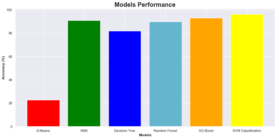
SVM classification has the highest accuracy score

Recommendation

SVM classification algorithm is the best modeling techinque for this project. This makes sense as the SVM methodology is the best technique for cluttered datasets with more than 3 dimensions. The data seems to be quite overlapping in 2D dimensions near the decision or classification boundaries (as seen in the 2D plots), but the SVM algorithm models the data at higher dimensions where the dataset can be linearly or distinctly divided into unique classes. Hence the higher scores.
But the disadvantage is that it is very time and resource consuming to run the SVM model. The XG Boost Model gives a comparable accuracy score and takes a lesser time to run the model.
The model can be further improved by eleminating or combining some of the correlated predictor variables like the (a) screen width and screen height, (b) pixel width and pixel height etc.
Model can also be simplified and improved by using just the RAM of the cell phones for classification purposes instead of all other variables as RAM alone contributes to almost 92% of the target classification (as per correlation matrix). To limit the scope of the analysis we have chosen not to implement Recommendations 3 & 4.

Project Risks

We have taken the 10 best features from the feature selection algorithm to reduce the dimensionality problem for modelling purposes, so if there are any interaction effects between the features that have not been modelled, due to lack of expertise in this field, there may be considerable amount of underperformance in the model when it is implemented.
The project assumes that the dataset used for modelling in this project is a representative of the population dataset else the models may not provide the accuracies that are shown here.