Telecom - Churn Rate ML

Project Team ID = PTID-CDS-JUL21-1171 (Members - Diana, Hema, Pavithra and Sophiya)

Project ID = PRCL-0017 Customer Churn Business case

—— Preliminary → Identify The Business Case ——

Project Description: No-Churn Telecom is an established Telecom operator in Europe with more than a decade in Business. Due to new players in the market, telecom industry has become very competitive and retaining customers becoming a challenge.
In spite of No-Churn initiatives of reducing tariffs and promoting more offers, the churn rate (percentage of customers migrating to competitors) is well above 10%.
No-Churn wants to explore the possibility of Machine Learning to help with following use cases to retain competitive edge in the industry.

Industry Field: Telecommunication Service
Project Goal → Help No-Churn with their use cases with ML

Understanding the variables that are influencing the customers to migrate.

Creating Churn risk scores that can be indicative to drive retention campaigns.

Introduce new predicting variable “CHURN-FLAG” with values YES(1) or NO(0) so that email campaigns with lucrative offers can be targeted to Churn YES customers.

Help to identify possible CHURN-FLAG YES customers and provide more attention in customer touch point areas, including customer care support, request fulfilment, auto categorizing tickets as high priority for quick resolutions any questions they may have etc.

png

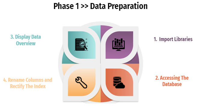png 1. Import Libraries

#!pip install ipython-sql --user
%reload_ext sql
from sqlalchemy import create_engine
import pandas as pd
#pip install PyMySQL --user
import pymysql
import numpy as np
import matplotlib.pyplot as plt
import seaborn as sns

import warnings
warnings.filterwarnings('ignore')

from sklearn.feature_selection import SelectKBest
from sklearn.feature_selection import chi2
from sklearn.model_selection import train_test_split
from sklearn.preprocessing import StandardScaler
from xgboost import plot_importance
from xgboost import XGBClassifier
#Importing libraries

from math import * # module math

from PIL import Image

import itertools
import io
import plotly.figure_factory as ff # visualization
import warnings
warnings.filterwarnings("ignore")
import os
from sklearn.metrics import confusion_matrix, accuracy_score, classification_report


import plotly.express as px
import plotly.graph_objects as go
import plotly.offline as py

2. Accessing The Database

db_host = '18.136.157.135'
username = 'dm_team3'
user_pass = 'DM!$!Team!27@9!20&'
db_name = 'project_telecom'

conn = create_engine('mysql+pymysql://'+username+':'+user_pass+'@'+db_host+'/'+db_name)
conn.table_names()

['telecom_churn_data']

query = "select * from telecom_churn_data" # SQL statement * --> selecting all columns and records
tcd = pd.read_sql(query,conn)
print(tcd.shape)
tcd.head()

(4617, 21)

	columns1	columns2	columns3	columns4	columns5	columns6	columns7	columns8	columns9	columns10	...	columns12	columns13	columns14	columns15	columns16	columns17	columns18	columns19	columns20	columns21
0	KS	128	415	382-4657	no	yes	25	265.1	110	45.07	...	99	16.78	244.7	91	11.01	10	3	2.7	1	False.
1	OH	107	415	371-7191	no	yes	26	161.6	123	27.47	...	103	16.62	254.4	103	11.45	13.7	3	3.7	1	False.
2	NJ	137	415	358-1921	no	no	0	243.4	114	41.38	...	110	10.3	162.6	104	7.32	12.2	5	3.29	0	False.
3	OH	84	408	375-9999	yes	no	0	299.4	71	50.9	...	88	5.26	196.9	89	8.86	6.6	7	1.78	2	False.
4	OK	75	415	330-6626	yes	no	0	166.7	113	28.34	...	122	12.61	186.9	121	8.41	10.1	3	2.73	3	False.

5 rows × 21 columns

3. Display Data Overview

#building function to cover data overview (data inspection)
def dataoveriew(df, message):
    print(f'{message}:\n')
    print("Rows:", df.shape[0])
    print("\nNumber of features:", df.shape[1])
    print("\nFeatures:")
    print(tcd.columns.tolist())
    print("\nMissing values:", df.isnull().sum().values.sum())
    print("\nUnique values:")
    print(df.nunique())
    print("\nDuplicated Rows:", df.duplicated().sum())
    print("\n____________________________________________")
    print("            Info of The Dataset")
    print("____________________________________________")
    print(df.info())

dataoveriew(tcd, 'Overiew of the dataset')

Overiew of the dataset:

Rows: 4617

Number of features: 21

Features:
['columns1', 'columns2', 'columns3', 'columns4', 'columns5', 'columns6', 'columns7', 'columns8', 'columns9', 'columns10', 'columns11', 'columns12', 'columns13', 'columns14', 'columns15', 'columns16', 'columns17', 'columns18', 'columns19', 'columns20', 'columns21']

Missing values: 0

Unique values:
columns1       51
columns2      218
columns3        3
columns4     4617
columns5        2
columns6        2
columns7       47
columns8     1901
columns9      123
columns10    1901
columns11    1833
columns12     125
columns13    1621
columns14    1813
columns15     130
columns16    1012
columns17     168
columns18      21
columns19     168
columns20      10
columns21       2
dtype: int64

Duplicated Rows: 0

____________________________________________
            Info of The Dataset
____________________________________________
<class 'pandas.core.frame.DataFrame'>
RangeIndex: 4617 entries, 0 to 4616
Data columns (total 21 columns):
 #   Column     Non-Null Count  Dtype 
---  ------     --------------  ----- 
 0   columns1   4617 non-null   object
 1   columns2   4617 non-null   object
 2   columns3   4617 non-null   object
 3   columns4   4617 non-null   object
 4   columns5   4617 non-null   object
 5   columns6   4617 non-null   object
 6   columns7   4617 non-null   object
 7   columns8   4617 non-null   object
 8   columns9   4617 non-null   object
 9   columns10  4617 non-null   object
 10  columns11  4617 non-null   object
 11  columns12  4617 non-null   object
 12  columns13  4617 non-null   object
 13  columns14  4617 non-null   object
 14  columns15  4617 non-null   object
 15  columns16  4617 non-null   object
 16  columns17  4617 non-null   object
 17  columns18  4617 non-null   object
 18  columns19  4617 non-null   object
 19  columns20  4617 non-null   object
 20  columns21  4617 non-null   object
dtypes: object(21)
memory usage: 757.6+ KB
None

As we can see above result, our data is pretty nice. No missing values inside, no duplicated rows.
Decision: move forward to rename the column

4. Rename Columns and Rectify The Index

#rename the columns as in pdf
dict = {'columns1':'State', 'columns2':'Account_Length', 'columns3':'Area_Code', 'columns4':'Phone', 'columns5':'International_Plan', 'columns6':'VMail_Plan', 'columns7':'VMail_Message',
        'columns8':'Day_Mins', 'columns9':'Day_Calls', 'columns10':'Day_Charge', 'columns11':'Eve_Mins', 'columns12':'Eve_Calls', 'columns13':'Eve_Charge', 'columns14':'Night_Mins', 
        'columns15':'Night_Calls', 'columns16':'Night_Charge', 'columns17':'International_Mins', 'columns18':'International_Calls', 'columns19':'International_Charge', 'columns20':'CustServ_Calls', 'columns21':'Churn'}

tcd.rename(columns = dict, inplace = True)

tcd.head()

	State	Account_Length	Area_Code	Phone	International_Plan	VMail_Plan	VMail_Message	Day_Mins	Day_Calls	Day_Charge	...	Eve_Calls	Eve_Charge	Night_Mins	Night_Calls	Night_Charge	International_Mins	International_Calls	International_Charge	CustServ_Calls	Churn
0	KS	128	415	382-4657	no	yes	25	265.1	110	45.07	...	99	16.78	244.7	91	11.01	10	3	2.7	1	False.
1	OH	107	415	371-7191	no	yes	26	161.6	123	27.47	...	103	16.62	254.4	103	11.45	13.7	3	3.7	1	False.
2	NJ	137	415	358-1921	no	no	0	243.4	114	41.38	...	110	10.3	162.6	104	7.32	12.2	5	3.29	0	False.
3	OH	84	408	375-9999	yes	no	0	299.4	71	50.9	...	88	5.26	196.9	89	8.86	6.6	7	1.78	2	False.
4	OK	75	415	330-6626	yes	no	0	166.7	113	28.34	...	122	12.61	186.9	121	8.41	10.1	3	2.73	3	False.

5 rows × 21 columns

# rectify the index
index = pd.Index(range(1, 4618))
tcd = tcd.set_index(index)
tcd.head()

	State	Account_Length	Area_Code	Phone	International_Plan	VMail_Plan	VMail_Message	Day_Mins	Day_Calls	Day_Charge	...	Eve_Calls	Eve_Charge	Night_Mins	Night_Calls	Night_Charge	International_Mins	International_Calls	International_Charge	CustServ_Calls	Churn
1	KS	128	415	382-4657	no	yes	25	265.1	110	45.07	...	99	16.78	244.7	91	11.01	10	3	2.7	1	False.
2	OH	107	415	371-7191	no	yes	26	161.6	123	27.47	...	103	16.62	254.4	103	11.45	13.7	3	3.7	1	False.
3	NJ	137	415	358-1921	no	no	0	243.4	114	41.38	...	110	10.3	162.6	104	7.32	12.2	5	3.29	0	False.
4	OH	84	408	375-9999	yes	no	0	299.4	71	50.9	...	88	5.26	196.9	89	8.86	6.6	7	1.78	2	False.
5	OK	75	415	330-6626	yes	no	0	166.7	113	28.34	...	122	12.61	186.9	121	8.41	10.1	3	2.73	3	False.

5 rows × 21 columns

tcd.describe().T

	count	unique	top	freq
State	4617	51	WV	149
Account_Length	4617	218	90	63
Area_Code	4617	3	415	2299
Phone	4617	4617	336-2113	1
International_Plan	4617	2	no	4171
VMail_Plan	4617	2	no	3381
VMail_Message	4617	47	0	3381
Day_Mins	4617	1901	154	10
Day_Calls	4617	123	102	108
Day_Charge	4617	1901	32.18	10
Eve_Mins	4617	1833	169.9	10
Eve_Calls	4617	125	105	111
Eve_Charge	4617	1621	14.25	15
Night_Mins	4617	1813	186.2	10
Night_Calls	4617	130	105	115
Night_Charge	4617	1012	9.66	19
International_Mins	4617	168	11.1	81
International_Calls	4617	21	3	925
International_Charge	4617	168	3	81
CustServ_Calls	4617	10	1	1651
Churn	4617	2	False.	3961

tcd.info()

<class 'pandas.core.frame.DataFrame'>
RangeIndex: 4617 entries, 1 to 4617
Data columns (total 21 columns):
 #   Column                Non-Null Count  Dtype 
---  ------                --------------  ----- 
 State                 4617 non-null   object
 Account_Length        4617 non-null   object
 Area_Code             4617 non-null   object
 Phone                 4617 non-null   object
 International_Plan    4617 non-null   object
 VMail_Plan            4617 non-null   object
 VMail_Message         4617 non-null   object
 Day_Mins              4617 non-null   object
 Day_Calls             4617 non-null   object
 Day_Charge            4617 non-null   object
Eve_Mins              4617 non-null   object
Eve_Calls             4617 non-null   object
Eve_Charge            4617 non-null   object
Night_Mins            4617 non-null   object
Night_Calls           4617 non-null   object
Night_Charge          4617 non-null   object
International_Mins    4617 non-null   object
International_Calls   4617 non-null   object
International_Charge  4617 non-null   object
CustServ_Calls        4617 non-null   object
Churn                 4617 non-null   object
dtypes: object(21)
memory usage: 757.6+ KB

As we can see above, the descriptive statistics result seems to be unproper served. Cause according to our tcd.info(), the entire variables data type are setted as ‘object’.
Decision: modify the dtypes of each variables according to .pdf (Project details) ___

tcd = tcd.astype({'Day_Mins': 'float64', 'Day_Charge': 'float64', 'Eve_Mins': 'float64', 'Eve_Charge': 'float64',
                    'Night_Mins': 'float64', 'Night_Charge': 'float64', 'International_Mins': 'float64', 'International_Charge': 'float64'})
#tcd.info()

tcd = tcd.astype({'Account_Length': 'int64', 'Area_Code': 'int64', 'VMail_Message': 'int64', 'Day_Calls': 'int64',
                    'Eve_Calls': 'int64', 'Night_Calls': 'int64', 'International_Calls': 'int64', 'CustServ_Calls':'int64'})
dataoveriew(tcd, 'Overiew of the dataset')

Overiew of the dataset:

Rows: 4617

Number of features: 21

Features:
['State', 'Account_Length', 'Area_Code', 'Phone', 'International_Plan', 'VMail_Plan', 'VMail_Message', 'Day_Mins', 'Day_Calls', 'Day_Charge', 'Eve_Mins', 'Eve_Calls', 'Eve_Charge', 'Night_Mins', 'Night_Calls', 'Night_Charge', 'International_Mins', 'International_Calls', 'International_Charge', 'CustServ_Calls', 'Churn']

Missing values: 0

Unique values:
State                     51
Account_Length           218
Area_Code                  3
Phone                   4617
International_Plan         2
VMail_Plan                 2
VMail_Message             47
Day_Mins                1901
Day_Calls                123
Day_Charge              1901
Eve_Mins                1833
Eve_Calls                125
Eve_Charge              1621
Night_Mins              1813
Night_Calls              130
Night_Charge            1012
International_Mins       168
International_Calls       21
International_Charge     168
CustServ_Calls            10
Churn                      2
dtype: int64

Duplicated Rows: 0

____________________________________________
            Info of The Dataset
____________________________________________
<class 'pandas.core.frame.DataFrame'>
RangeIndex: 4617 entries, 1 to 4617
Data columns (total 21 columns):
 #   Column                Non-Null Count  Dtype  
---  ------                --------------  -----  
 0   State                 4617 non-null   object 
 1   Account_Length        4617 non-null   int64  
 2   Area_Code             4617 non-null   int64  
 3   Phone                 4617 non-null   object 
 4   International_Plan    4617 non-null   object 
 5   VMail_Plan            4617 non-null   object 
 6   VMail_Message         4617 non-null   int64  
 7   Day_Mins              4617 non-null   float64
 8   Day_Calls             4617 non-null   int64  
 9   Day_Charge            4617 non-null   float64
 10  Eve_Mins              4617 non-null   float64
 11  Eve_Calls             4617 non-null   int64  
 12  Eve_Charge            4617 non-null   float64
 13  Night_Mins            4617 non-null   float64
 14  Night_Calls           4617 non-null   int64  
 15  Night_Charge          4617 non-null   float64
 16  International_Mins    4617 non-null   float64
 17  International_Calls   4617 non-null   int64  
 18  International_Charge  4617 non-null   float64
 19  CustServ_Calls        4617 non-null   int64  
 20  Churn                 4617 non-null   object 
dtypes: float64(8), int64(8), object(5)
memory usage: 757.6+ KB
None

Some of dtypes has been changed. Go forward to show descriptive statistics

tcd.describe().T

	count	mean	std	min	25%	50%	75%	max
Account_Length	4617.0	100.645224	39.597194	1.00	74.00	100.00	127.00	243.00
Area_Code	4617.0	437.046350	42.288212	408.00	408.00	415.00	510.00	510.00
VMail_Message	4617.0	7.849903	13.592333	0.00	0.00	0.00	17.00	51.00
Day_Mins	4617.0	180.447152	53.983540	0.00	143.70	180.00	216.80	351.50
Day_Calls	4617.0	100.054364	19.883027	0.00	87.00	100.00	113.00	165.00
Day_Charge	4617.0	30.676576	9.177145	0.00	24.43	30.60	36.86	59.76
Eve_Mins	4617.0	200.429088	50.557001	0.00	165.90	200.80	234.00	363.70
Eve_Calls	4617.0	100.179770	19.821314	0.00	87.00	101.00	114.00	170.00
Eve_Charge	4617.0	17.036703	4.297332	0.00	14.10	17.07	19.89	30.91
Night_Mins	4617.0	200.623933	50.543616	23.20	167.10	200.80	234.90	395.00
Night_Calls	4617.0	99.944120	19.935053	12.00	87.00	100.00	113.00	175.00
Night_Charge	4617.0	9.028185	2.274488	1.04	7.52	9.04	10.57	17.77
International_Mins	4617.0	10.279294	2.757361	0.00	8.60	10.30	12.10	20.00
International_Calls	4617.0	4.433831	2.457615	0.00	3.00	4.00	6.00	20.00
International_Charge	4617.0	2.775926	0.744413	0.00	2.32	2.78	3.27	5.40
CustServ_Calls	4617.0	1.567035	1.307019	0.00	1.00	1.00	2.00	9.00

So far is good, just need a little touch up to handling categorical values.
Decision: go forward to encoding ‘object’ dtypes to covering the entire columns. So the descriptive statistics above would involving the whole features.

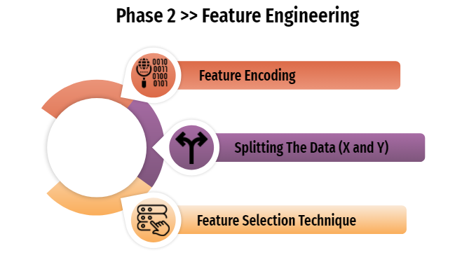png 1. Feature Encoding

from sklearn.preprocessing import LabelEncoder

#build function to encoding multiple variables (object dtype)
class MultiColumnLabelEncoder:
    def __init__(self,columns = None):
        self.columns = columns # array of column names to encode

    def fit(self,X,y=None):
        return self #

    def transform(self,X):
        '''
        Transforms columns of X specified in self.columns using
        LabelEncoder(). If no columns specified, transforms all
        columns in X.
        '''
        output = X.copy()
        if self.columns is not None:
            for col in self.columns:
                output[col] = LabelEncoder().fit_transform(output[col])
        else:
            for colname,col in output.iteritems():
                output[colname] = LabelEncoder().fit_transform(col)
        return output

    def fit_transform(self,X,y=None):
        return self.fit(X,y).transform(X)

MultiColumnLabelEncoder(columns = ['State','Phone', 'International_Plan', 'VMail_Plan', 'Churn']).fit_transform(tcd)

	State	Account_Length	Area_Code	Phone	International_Plan	VMail_Plan	VMail_Message	Day_Mins	Day_Calls	Day_Charge	...	Eve_Calls	Eve_Charge	Night_Mins	Night_Calls	Night_Charge	International_Mins	International_Calls	International_Charge	CustServ_Calls	Churn
1	16	128	415	2637	0	1	25	265.1	110	45.07	...	99	16.78	244.7	91	11.01	10.0	3	2.70	1	0
2	35	107	415	2132	0	1	26	161.6	123	27.47	...	103	16.62	254.4	103	11.45	13.7	3	3.70	1	0
3	31	137	415	1509	0	0	0	243.4	114	41.38	...	110	10.30	162.6	104	7.32	12.2	5	3.29	0	0
4	35	84	408	2326	1	0	0	299.4	71	50.90	...	88	5.26	196.9	89	8.86	6.6	7	1.78	2	0
5	36	75	415	150	1	0	0	166.7	113	28.34	...	122	12.61	186.9	121	8.41	10.1	3	2.73	3	0
...	...	...	...	...	...	...	...	...	...	...	...	...	...	...	...	...	...	...	...	...	...
4613	34	57	510	890	0	1	25	144.0	81	24.48	...	112	15.91	158.6	122	7.14	8.5	6	2.30	3	0
4614	32	177	408	795	0	1	29	189.0	91	32.13	...	96	25.76	163.6	116	7.36	15.7	1	4.24	3	0
4615	46	67	408	533	0	1	33	127.5	126	21.68	...	129	25.17	200.9	91	9.04	13.0	3	3.51	1	0
4616	22	98	415	1406	0	1	23	168.9	98	28.71	...	117	19.24	165.5	96	7.45	14.3	3	3.86	0	0
4617	15	140	415	4013	0	0	0	204.7	100	34.80	...	107	10.78	202.8	115	9.13	12.1	4	3.27	2	0

4617 rows × 21 columns

tcd = MultiColumnLabelEncoder(columns = ['State','Phone', 'International_Plan', 'VMail_Plan', 'Churn']).fit_transform(tcd)

tcd.describe().T

	count	mean	std	min	25%	50%	75%	max
State	4617.0	26.041585	14.790361	0.00	13.00	26.00	39.00	50.00
Account_Length	4617.0	100.645224	39.597194	1.00	74.00	100.00	127.00	243.00
Area_Code	4617.0	437.046350	42.288212	408.00	408.00	415.00	510.00	510.00
Phone	4617.0	2308.000000	1332.957426	0.00	1154.00	2308.00	3462.00	4616.00
International_Plan	4617.0	0.096600	0.295444	0.00	0.00	0.00	0.00	1.00
VMail_Plan	4617.0	0.267706	0.442812	0.00	0.00	0.00	1.00	1.00
VMail_Message	4617.0	7.849903	13.592333	0.00	0.00	0.00	17.00	51.00
Day_Mins	4617.0	180.447152	53.983540	0.00	143.70	180.00	216.80	351.50
Day_Calls	4617.0	100.054364	19.883027	0.00	87.00	100.00	113.00	165.00
Day_Charge	4617.0	30.676576	9.177145	0.00	24.43	30.60	36.86	59.76
Eve_Mins	4617.0	200.429088	50.557001	0.00	165.90	200.80	234.00	363.70
Eve_Calls	4617.0	100.179770	19.821314	0.00	87.00	101.00	114.00	170.00
Eve_Charge	4617.0	17.036703	4.297332	0.00	14.10	17.07	19.89	30.91
Night_Mins	4617.0	200.623933	50.543616	23.20	167.10	200.80	234.90	395.00
Night_Calls	4617.0	99.944120	19.935053	12.00	87.00	100.00	113.00	175.00
Night_Charge	4617.0	9.028185	2.274488	1.04	7.52	9.04	10.57	17.77
International_Mins	4617.0	10.279294	2.757361	0.00	8.60	10.30	12.10	20.00
International_Calls	4617.0	4.433831	2.457615	0.00	3.00	4.00	6.00	20.00
International_Charge	4617.0	2.775926	0.744413	0.00	2.32	2.78	3.27	5.40
CustServ_Calls	4617.0	1.567035	1.307019	0.00	1.00	1.00	2.00	9.00
Churn	4617.0	0.142084	0.349174	0.00	0.00	0.00	0.00	1.00

Fabulous.. they’re involving the entire columns (variables) inside our dataframe, no mess in between.
Decision: go forward into the next step.

2. Splitting The Data (X and Y)

# splitting the data into X and Y so we can do feature selection / feature importance

x = tcd.drop('Churn', axis=1)
y = tcd['Churn']
display(x.head())
display(y.head())

	State	Account_Length	Area_Code	Phone	International_Plan	VMail_Plan	VMail_Message	Day_Mins	Day_Calls	Day_Charge	Eve_Mins	Eve_Calls	Eve_Charge	Night_Mins	Night_Calls	Night_Charge	International_Mins	International_Calls	International_Charge	CustServ_Calls
1	16	128	415	2637	0	1	25	265.1	110	45.07	197.4	99	16.78	244.7	91	11.01	10.0	3	2.70	1
2	35	107	415	2132	0	1	26	161.6	123	27.47	195.5	103	16.62	254.4	103	11.45	13.7	3	3.70	1
3	31	137	415	1509	0	0	0	243.4	114	41.38	121.2	110	10.30	162.6	104	7.32	12.2	5	3.29	0
4	35	84	408	2326	1	0	0	299.4	71	50.90	61.9	88	5.26	196.9	89	8.86	6.6	7	1.78	2
5	36	75	415	150	1	0	0	166.7	113	28.34	148.3	122	12.61	186.9	121	8.41	10.1	3	2.73	3

  0
  0
  0
  0
  0
Name: Churn, dtype: int32

To narrow the scope, we agreed to limit 10 features at the modeling stage. 10 features are selected based on feature selection techniques and top 10 rankings. This is done to prevent "the curse of dimensionality" which will lead to overfitting.

3. Feature Selection Technique

# FEATURE SELECTION TECHNIQUE
#apply SelectKBest class to extract top 10 best features
bestfeatures = SelectKBest(score_func=chi2, k=10)
fit = bestfeatures.fit(x,y)
dfscores = pd.DataFrame(fit.scores_)
dfcolumns = pd.DataFrame(x.columns)

#concat two dataframes for better visualization
featurescores = pd.concat([dfcolumns,dfscores], axis=1)
featurescores.columns = ['Specs', 'Score'] #naming the data
print(featurescores.nlargest(10, 'Score'))

                 Specs        Score
           Day_Mins  3055.100135
      VMail_Message  1019.757912
         Day_Charge   519.329000
          Eve_Mins   445.993054
 International_Plan   276.614354
              Phone   276.402610
    CustServ_Calls   220.546005
        Night_Mins   110.011675
         VMail_Plan    41.021084
        Eve_Charge    37.902981

According to the result above, it is proven that 10 selected features could be able to influence the "churn rate", it designates that customers-decision whether they decide to keep stay (subscribe) or migrate. [Project Goal Number 1 Solved]

#applied selected feature above to our X variables (features)

X = x[['Day_Mins', 'VMail_Message', 'Day_Charge','Eve_Mins','International_Plan','Phone','CustServ_Calls','Night_Mins','VMail_Plan','Eve_Charge']].copy()
X.head()

	Day_Mins	VMail_Message	Day_Charge	Eve_Mins	International_Plan	Phone	CustServ_Calls	Night_Mins	VMail_Plan	Eve_Charge
1	265.1	25	45.07	197.4	0	2637	1	244.7	1	16.78
2	161.6	26	27.47	195.5	0	2132	1	254.4	1	16.62
3	243.4	0	41.38	121.2	0	1509	0	162.6	0	10.30
4	299.4	0	50.90	61.9	1	2326	2	196.9	0	5.26
5	166.7	0	28.34	148.3	1	150	3	186.9	0	12.61

Final result will be use to perpetuate to further phase.

png

This phase purpose is to get the insight and understand of our data. Whether it needs further treatment or not, it will be checked on this phase to prevent any mistakes in a further steps.

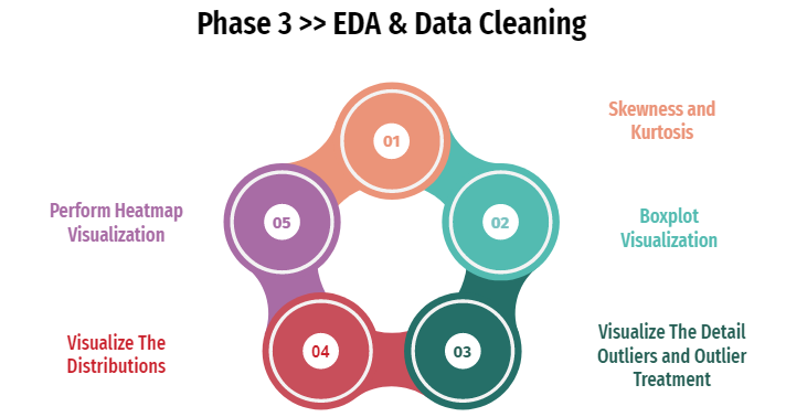
1. Skewness and Kurtosis

display('--- Skewness of 10 Selected Features ---',X.skew())
display('--- Kurtosis of 10 Selected Festures ---',X.kurtosis())

'--- Skewness of 10 Selected Features ---'



Day_Mins             -0.002948
VMail_Message         1.326734
Day_Charge           -0.002952
Eve_Mins             -0.005280
International_Plan    2.731995
Phone                 0.000000
CustServ_Calls        1.046800
Night_Mins            0.020515
VMail_Plan            1.049631
Eve_Charge           -0.005252
dtype: float64



'--- Kurtosis of 10 Selected Festures ---'



Day_Mins             -0.042399
VMail_Message         0.123526
Day_Charge           -0.042264
Eve_Mins              0.043630
International_Plan    5.466164
Phone                -1.200000
CustServ_Calls        1.515026
Night_Mins            0.061409
VMail_Plan           -0.898664
Eve_Charge            0.043522
dtype: float64

2. Boxplot Visualization

#Boxplot analysis

figure, ax = plt.subplots(2,5, figsize=(20,10))


plt.suptitle('Boxplot of 10 Selected Features', size = 20)
sns.boxplot(X['Day_Mins'],ax=ax[0,0])
sns.boxplot(X['VMail_Message'], ax=ax[0,1])
sns.boxplot(X['Day_Charge'], ax=ax[0,2])
sns.boxplot(X['Eve_Mins'], ax=ax[0,3])
sns.boxplot(X['International_Plan'], ax=ax[0,4])
sns.boxplot(X['Phone'], ax=ax[1,0])
sns.boxplot(X['CustServ_Calls'], ax=ax[1,1])
sns.boxplot(X['Night_Mins'], ax=ax[1,2])
sns.boxplot(X['VMail_Plan'], ax=ax[1,3])
sns.boxplot(X['Eve_Charge'], ax=ax[1,4])
#plt.savefig('[Fig 3.1] Boxplot of 10 Selected Features.png', dpi = 300)
plt.show()

png

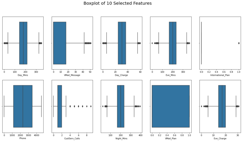
From visualization above, we found a lot of outliers almost in every 10 selected features (except for 'Phone' and 'Vmail_Plan').
Decision: move forward into the details, which will show the exact values that fall into the outlier category.

3. Visualize The Detail Outliers and Outlier Treatment

def outliers_detection_result(data):
    # Counting Q1 & Q3 values
    Q1 = np.quantile(data, .25)
    Q3 = np.quantile(data, .75)
    IQR = Q3 - Q1
    print('Quartile 1 = ', Q1)
    print('Quartile 3 = ', Q3)
    print('IQR = ', IQR)
    min_IQR = Q1 - 1.5 * IQR
    max_IQR = Q3 + 1.5 * IQR
    
    print('Minimum IQR = ', min_IQR)
    print('Maximum IQR = ', max_IQR)

    min_values = np.min(data)
    max_values = np.max(data)

    print('Minimum value = ', min_values)
    print('Maximum value = ', max_values)
    if (min_values < min_IQR):
        print('Found low outlier!')
    else:
        print('Not found low outlier!')  

    if (max_values > max_IQR):
        print('Found high outlier!')
    else:
        print('Not found high outlier!')

    low_out = []
    high_out = []

    for i in data:
        if (i < min_IQR):
            low_out.append(i)
        if (i > max_IQR):
            high_out.append(i)

    print('Low outlier : ', low_out)
    print('High outlier : ', high_out)

print('------------------ 1. Day_Mins Outliers Detection: ------------------')
outliers_detection_result(X.Day_Mins)
print('\n------------------ 2. VMail_Message Outliers Detection: ------------------')
outliers_detection_result(X.VMail_Message)
print('\n------------------ 3. Day_Charge Outliers Detection: ------------------')
outliers_detection_result(X.Day_Charge)
print('\n------------------ 4. Eve_Mins Outliers Detection: ------------------')
outliers_detection_result(X.Eve_Mins)
print('\n------------------ 5. International_Plan Outliers Detection: ------------------')
outliers_detection_result(X.International_Plan)
print('\n------------------ 6. Phone Outliers Detection: ------------------')
outliers_detection_result(X.Phone)
print('\n------------------ 7. CustServ_Calls Outliers Detection: ------------------')
outliers_detection_result(X.CustServ_Calls)
print('\n------------------ 8. Night_Mins Outliers Detection: ------------------')
outliers_detection_result(X.Night_Mins)
print('\n------------------ 9. VMail_Plan Outliers Detection: ------------------')
outliers_detection_result(X.VMail_Plan)
print('\n------------------ 10. Eve_Charge Outliers Detection: ------------------')
outliers_detection_result(X.Eve_Charge)

------------------ 1. Day_Mins Outliers Detection: ------------------
Quartile 1 =  143.7
Quartile 3 =  216.8
IQR =  73.10000000000002
Minimum IQR =  34.049999999999955
Maximum IQR =  326.45000000000005
Minimum value =  0.0
Maximum value =  351.5
Found low outlier!
Found high outlier!
Low outlier :  [30.9, 34.0, 12.5, 25.9, 0.0, 0.0, 19.5, 7.9, 27.0, 17.6, 2.6, 7.8, 18.9, 29.9]
High outlier :  [332.9, 337.4, 326.5, 350.8, 335.5, 334.3, 346.8, 329.8, 328.1, 345.3, 338.4, 351.5, 332.1]

------------------ 2. VMail_Message Outliers Detection: ------------------
Quartile 1 =  0.0
Quartile 3 =  17.0
IQR =  17.0
Minimum IQR =  -25.5
Maximum IQR =  42.5
Minimum value =  0
Maximum value =  51
Not found low outlier!
Found high outlier!
Low outlier :  []
High outlier :  [46, 43, 48, 48, 45, 46, 43, 45, 51, 43, 45, 46, 43, 47, 44, 44, 49, 44, 43, 47, 43, 45, 45, 45, 43, 46, 44, 50, 44, 50, 47, 44, 43, 44, 43, 43, 46, 45, 49, 46, 49, 45, 43, 47, 46, 45, 43, 46, 45, 48, 43]

------------------ 3. Day_Charge Outliers Detection: ------------------
Quartile 1 =  24.43
Quartile 3 =  36.86
IQR =  12.43
Minimum IQR =  5.785
Maximum IQR =  55.504999999999995
Minimum value =  0.0
Maximum value =  59.76
Found low outlier!
Found high outlier!
Low outlier :  [5.25, 5.78, 2.13, 4.4, 0.0, 0.0, 3.32, 1.34, 4.59, 2.99, 0.44, 1.33, 3.21, 5.08]
High outlier :  [56.59, 57.36, 55.51, 59.64, 57.04, 56.83, 58.96, 56.07, 55.78, 58.7, 57.53, 59.76, 56.46]

------------------ 4. Eve_Mins Outliers Detection: ------------------
Quartile 1 =  165.9
Quartile 3 =  234.0
IQR =  68.1
Minimum IQR =  63.750000000000014
Maximum IQR =  336.15
Minimum value =  0.0
Maximum value =  363.7
Found low outlier!
Found high outlier!
Low outlier :  [61.9, 31.2, 42.2, 58.9, 43.9, 52.9, 42.5, 60.8, 58.6, 56.0, 48.1, 60.0, 49.2, 0.0, 22.3, 58.3, 37.8, 41.7, 47.3, 53.2]
High outlier :  [348.5, 351.6, 350.5, 337.1, 347.3, 350.9, 339.9, 361.8, 354.2, 363.7, 341.3, 344.0, 349.4, 348.9, 344.9, 352.1]

------------------ 5. International_Plan Outliers Detection: ------------------
Quartile 1 =  0.0
Quartile 3 =  0.0
IQR =  0.0
Minimum IQR =  0.0
Maximum IQR =  0.0
Minimum value =  0
Maximum value =  1
Not found low outlier!
Found high outlier!
Low outlier :  []
High outlier :  [1, 1, 1, 1, 1, 1, 1, 1, 1, 1, 1, 1, 1, 1, 1, 1, 1, 1, 1, 1, 1, 1, 1, 1, 1, 1, 1, 1, 1, 1, 1, 1, 1, 1, 1, 1, 1, 1, 1, 1, 1, 1, 1, 1, 1, 1, 1, 1, 1, 1, 1, 1, 1, 1, 1, 1, 1, 1, 1, 1, 1, 1, 1, 1, 1, 1, 1, 1, 1, 1, 1, 1, 1, 1, 1, 1, 1, 1, 1, 1, 1, 1, 1, 1, 1, 1, 1, 1, 1, 1, 1, 1, 1, 1, 1, 1, 1, 1, 1, 1, 1, 1, 1, 1, 1, 1, 1, 1, 1, 1, 1, 1, 1, 1, 1, 1, 1, 1, 1, 1, 1, 1, 1, 1, 1, 1, 1, 1, 1, 1, 1, 1, 1, 1, 1, 1, 1, 1, 1, 1, 1, 1, 1, 1, 1, 1, 1, 1, 1, 1, 1, 1, 1, 1, 1, 1, 1, 1, 1, 1, 1, 1, 1, 1, 1, 1, 1, 1, 1, 1, 1, 1, 1, 1, 1, 1, 1, 1, 1, 1, 1, 1, 1, 1, 1, 1, 1, 1, 1, 1, 1, 1, 1, 1, 1, 1, 1, 1, 1, 1, 1, 1, 1, 1, 1, 1, 1, 1, 1, 1, 1, 1, 1, 1, 1, 1, 1, 1, 1, 1, 1, 1, 1, 1, 1, 1, 1, 1, 1, 1, 1, 1, 1, 1, 1, 1, 1, 1, 1, 1, 1, 1, 1, 1, 1, 1, 1, 1, 1, 1, 1, 1, 1, 1, 1, 1, 1, 1, 1, 1, 1, 1, 1, 1, 1, 1, 1, 1, 1, 1, 1, 1, 1, 1, 1, 1, 1, 1, 1, 1, 1, 1, 1, 1, 1, 1, 1, 1, 1, 1, 1, 1, 1, 1, 1, 1, 1, 1, 1, 1, 1, 1, 1, 1, 1, 1, 1, 1, 1, 1, 1, 1, 1, 1, 1, 1, 1, 1, 1, 1, 1, 1, 1, 1, 1, 1, 1, 1, 1, 1, 1, 1, 1, 1, 1, 1, 1, 1, 1, 1, 1, 1, 1, 1, 1, 1, 1, 1, 1, 1, 1, 1, 1, 1, 1, 1, 1, 1, 1, 1, 1, 1, 1, 1, 1, 1, 1, 1, 1, 1, 1, 1, 1, 1, 1, 1, 1, 1, 1, 1, 1, 1, 1, 1, 1, 1, 1, 1, 1, 1, 1, 1, 1, 1, 1, 1, 1, 1, 1, 1, 1, 1, 1, 1, 1, 1, 1, 1, 1, 1, 1, 1, 1, 1, 1, 1, 1, 1, 1, 1, 1, 1, 1, 1, 1, 1, 1, 1, 1, 1, 1, 1, 1, 1, 1, 1, 1, 1, 1, 1, 1, 1, 1, 1, 1, 1]

------------------ 6. Phone Outliers Detection: ------------------
Quartile 1 =  1154.0
Quartile 3 =  3462.0
IQR =  2308.0
Minimum IQR =  -2308.0
Maximum IQR =  6924.0
Minimum value =  0
Maximum value =  4616
Not found low outlier!
Not found high outlier!
Low outlier :  []
High outlier :  []

------------------ 7. CustServ_Calls Outliers Detection: ------------------
Quartile 1 =  1.0
Quartile 3 =  2.0
IQR =  1.0
Minimum IQR =  -0.5
Maximum IQR =  3.5
Minimum value =  0
Maximum value =  9
Not found low outlier!
Found high outlier!
Low outlier :  []
High outlier :  [4, 4, 4, 5, 5, 5, 4, 4, 4, 4, 4, 4, 4, 4, 4, 4, 5, 5, 4, 5, 4, 4, 5, 4, 4, 4, 4, 4, 5, 4, 4, 7, 4, 4, 4, 4, 4, 5, 4, 4, 4, 4, 4, 5, 4, 7, 4, 9, 5, 4, 4, 5, 4, 4, 5, 5, 4, 6, 4, 6, 5, 5, 5, 6, 5, 4, 4, 5, 4, 4, 7, 4, 6, 5, 4, 4, 4, 6, 4, 4, 5, 4, 4, 4, 4, 4, 4, 5, 5, 6, 5, 4, 4, 4, 5, 4, 4, 4, 4, 5, 5, 4, 4, 4, 4, 6, 4, 5, 4, 6, 4, 4, 4, 4, 4, 4, 4, 4, 4, 6, 4, 4, 4, 4, 8, 4, 4, 5, 4, 4, 4, 6, 5, 5, 7, 4, 4, 5, 4, 4, 5, 4, 4, 5, 7, 4, 4, 5, 7, 4, 4, 4, 4, 8, 6, 4, 4, 5, 5, 5, 4, 4, 5, 4, 4, 4, 4, 4, 4, 4, 4, 4, 4, 5, 6, 4, 5, 4, 4, 5, 5, 4, 6, 4, 4, 4, 9, 6, 4, 5, 5, 4, 6, 4, 4, 5, 4, 4, 4, 5, 5, 6, 4, 5, 4, 4, 4, 4, 5, 4, 4, 4, 5, 4, 5, 6, 4, 4, 5, 4, 4, 4, 5, 4, 4, 4, 4, 4, 5, 7, 6, 5, 6, 7, 5, 5, 4, 6, 4, 4, 4, 4, 5, 6, 7, 4, 4, 4, 5, 5, 5, 4, 4, 4, 5, 6, 5, 5, 4, 4, 4, 4, 4, 4, 4, 4, 5, 4, 4, 5, 5, 4, 4, 5, 4, 5, 4, 4, 4, 5, 5, 4, 4, 6, 6, 4, 5, 5, 4, 4, 5, 4, 5, 4, 5, 4, 4, 4, 4, 4, 4, 4, 4, 4, 4, 6, 4, 4, 4, 4, 5, 4, 4, 4, 5, 5, 4, 4, 5, 5, 5, 4, 4, 7, 4, 4, 5, 5, 5, 6, 4, 4, 4, 4, 4, 4, 4, 4, 4, 4, 4, 7, 7, 4, 6, 4, 4, 4, 4, 4, 4, 4, 4, 4, 7, 5, 4, 4, 4, 5, 4, 4, 6, 4, 4, 5, 4, 4]

------------------ 8. Night_Mins Outliers Detection: ------------------
Quartile 1 =  167.1
Quartile 3 =  234.9
IQR =  67.80000000000001
Minimum IQR =  65.39999999999998
Maximum IQR =  336.6
Minimum value =  23.2
Maximum value =  395.0
Found low outlier!
Found high outlier!
Low outlier :  [57.5, 45.0, 63.3, 54.5, 50.1, 43.7, 23.2, 63.6, 56.6, 54.0, 64.2, 50.1, 53.3, 61.4, 47.4, 50.9, 46.7, 65.2, 59.5]
High outlier :  [354.9, 349.2, 345.8, 342.8, 364.3, 349.7, 352.5, 381.9, 377.5, 367.7, 344.3, 395.0, 350.2, 352.2, 364.9, 381.6, 359.9]

------------------ 9. VMail_Plan Outliers Detection: ------------------
Quartile 1 =  0.0
Quartile 3 =  1.0
IQR =  1.0
Minimum IQR =  -1.5
Maximum IQR =  2.5
Minimum value =  0
Maximum value =  1
Not found low outlier!
Not found high outlier!
Low outlier :  []
High outlier :  []

------------------ 10. Eve_Charge Outliers Detection: ------------------
Quartile 1 =  14.1
Quartile 3 =  19.89
IQR =  5.790000000000001
Minimum IQR =  5.414999999999997
Maximum IQR =  28.575000000000003
Minimum value =  0.0
Maximum value =  30.91
Found low outlier!
Found high outlier!
Low outlier :  [5.26, 2.65, 3.59, 5.01, 3.73, 4.5, 3.61, 5.17, 4.98, 4.76, 4.09, 5.1, 4.18, 0.0, 1.9, 4.96, 3.21, 3.54, 4.02, 4.52]
High outlier :  [29.62, 29.89, 29.79, 28.65, 29.52, 29.83, 28.89, 30.75, 30.11, 30.91, 29.01, 29.24, 29.7, 29.66, 29.32, 29.93]

That’s the details of outliers on each features.
Decision: treat outliers by replacing them with 95th and 5th percentile.

#build functions (outliers treatment) by replacing them with the 95th and 5th percentile.
def outliers_treatment(df, field_name):
    p_05 = df[field_name].quantile(0.05) # 5th quantile
    p_95 = df[field_name].quantile(0.95) # 95th quantile
    df[field_name].clip(p_05, p_95, inplace=True)
    print('Status: Completed\n')
    print('------------------- Report -------------------')
    outliers_detection_result(df[field_name])
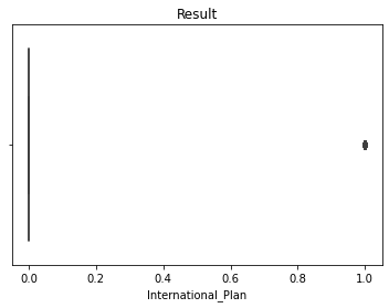
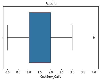
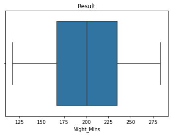
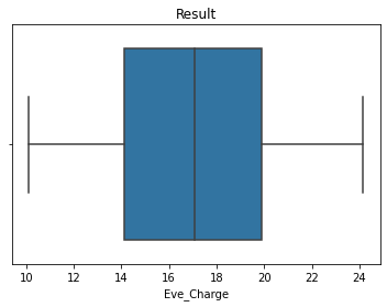
    sns.boxplot(df[field_name])
    plt.title('Result')
    plt.show()

display(outliers_treatment(X, 'Day_Mins'))
display(outliers_treatment(X, 'VMail_Message'))
display(outliers_treatment(X, 'Day_Charge'))
display(outliers_treatment(X, 'Eve_Mins'))
display(outliers_treatment(X, 'International_Plan'))
display(outliers_treatment(X, 'CustServ_Calls'))
display(outliers_treatment(X, 'Night_Mins'))
display(outliers_treatment(X, 'Eve_Charge'))

Status: Completed

------------------- Report -------------------
Quartile 1 =  143.7
Quartile 3 =  216.8
IQR =  73.10000000000002
Minimum IQR =  34.049999999999955
Maximum IQR =  326.45000000000005
Minimum value =  91.66000000000001
Maximum value =  271.1
Not found low outlier!
Not found high outlier!
Low outlier :  []
High outlier :  []

png

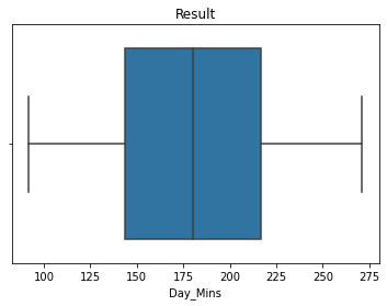
None


Status: Completed

------------------- Report -------------------
Quartile 1 =  0.0
Quartile 3 =  17.0
IQR =  17.0
Minimum IQR =  -25.5
Maximum IQR =  42.5
Minimum value =  0
Maximum value =  37
Not found low outlier!
Not found high outlier!
Low outlier :  []
High outlier :  []

png

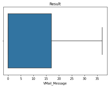
None


Status: Completed

------------------- Report -------------------
Quartile 1 =  24.43
Quartile 3 =  36.86
IQR =  12.43
Minimum IQR =  5.785
Maximum IQR =  55.504999999999995
Minimum value =  15.584
Maximum value =  46.09
Not found low outlier!
Not found high outlier!
Low outlier :  []
High outlier :  []

png

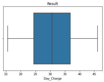
None


Status: Completed

------------------- Report -------------------
Quartile 1 =  165.9
Quartile 3 =  234.0
IQR =  68.1
Minimum IQR =  63.750000000000014
Maximum IQR =  336.15
Minimum value =  118.78
Maximum value =  284.12
Not found low outlier!
Not found high outlier!
Low outlier :  []
High outlier :  []

png

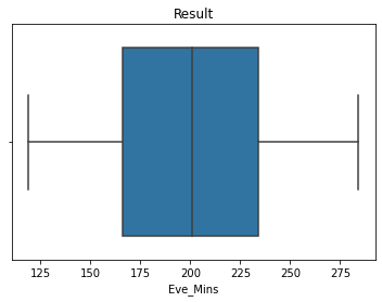
None


Status: Completed

------------------- Report -------------------
Quartile 1 =  0.0
Quartile 3 =  0.0
IQR =  0.0
Minimum IQR =  0.0
Maximum IQR =  0.0
Minimum value =  0
Maximum value =  1
Not found low outlier!
Found high outlier!
Low outlier :  []
High outlier :  [1, 1, 1, 1, 1, 1, 1, 1, 1, 1, 1, 1, 1, 1, 1, 1, 1, 1, 1, 1, 1, 1, 1, 1, 1, 1, 1, 1, 1, 1, 1, 1, 1, 1, 1, 1, 1, 1, 1, 1, 1, 1, 1, 1, 1, 1, 1, 1, 1, 1, 1, 1, 1, 1, 1, 1, 1, 1, 1, 1, 1, 1, 1, 1, 1, 1, 1, 1, 1, 1, 1, 1, 1, 1, 1, 1, 1, 1, 1, 1, 1, 1, 1, 1, 1, 1, 1, 1, 1, 1, 1, 1, 1, 1, 1, 1, 1, 1, 1, 1, 1, 1, 1, 1, 1, 1, 1, 1, 1, 1, 1, 1, 1, 1, 1, 1, 1, 1, 1, 1, 1, 1, 1, 1, 1, 1, 1, 1, 1, 1, 1, 1, 1, 1, 1, 1, 1, 1, 1, 1, 1, 1, 1, 1, 1, 1, 1, 1, 1, 1, 1, 1, 1, 1, 1, 1, 1, 1, 1, 1, 1, 1, 1, 1, 1, 1, 1, 1, 1, 1, 1, 1, 1, 1, 1, 1, 1, 1, 1, 1, 1, 1, 1, 1, 1, 1, 1, 1, 1, 1, 1, 1, 1, 1, 1, 1, 1, 1, 1, 1, 1, 1, 1, 1, 1, 1, 1, 1, 1, 1, 1, 1, 1, 1, 1, 1, 1, 1, 1, 1, 1, 1, 1, 1, 1, 1, 1, 1, 1, 1, 1, 1, 1, 1, 1, 1, 1, 1, 1, 1, 1, 1, 1, 1, 1, 1, 1, 1, 1, 1, 1, 1, 1, 1, 1, 1, 1, 1, 1, 1, 1, 1, 1, 1, 1, 1, 1, 1, 1, 1, 1, 1, 1, 1, 1, 1, 1, 1, 1, 1, 1, 1, 1, 1, 1, 1, 1, 1, 1, 1, 1, 1, 1, 1, 1, 1, 1, 1, 1, 1, 1, 1, 1, 1, 1, 1, 1, 1, 1, 1, 1, 1, 1, 1, 1, 1, 1, 1, 1, 1, 1, 1, 1, 1, 1, 1, 1, 1, 1, 1, 1, 1, 1, 1, 1, 1, 1, 1, 1, 1, 1, 1, 1, 1, 1, 1, 1, 1, 1, 1, 1, 1, 1, 1, 1, 1, 1, 1, 1, 1, 1, 1, 1, 1, 1, 1, 1, 1, 1, 1, 1, 1, 1, 1, 1, 1, 1, 1, 1, 1, 1, 1, 1, 1, 1, 1, 1, 1, 1, 1, 1, 1, 1, 1, 1, 1, 1, 1, 1, 1, 1, 1, 1, 1, 1, 1, 1, 1, 1, 1, 1, 1, 1, 1, 1, 1, 1, 1, 1, 1, 1, 1, 1, 1, 1, 1, 1, 1, 1, 1, 1, 1, 1, 1, 1, 1, 1, 1, 1, 1, 1, 1, 1, 1, 1, 1]

png

None


Status: Completed

------------------- Report -------------------
Quartile 1 =  1.0
Quartile 3 =  2.0
IQR =  1.0
Minimum IQR =  -0.5
Maximum IQR =  3.5
Minimum value =  0
Maximum value =  4
Not found low outlier!
Found high outlier!
Low outlier :  []
High outlier :  [4, 4, 4, 4, 4, 4, 4, 4, 4, 4, 4, 4, 4, 4, 4, 4, 4, 4, 4, 4, 4, 4, 4, 4, 4, 4, 4, 4, 4, 4, 4, 4, 4, 4, 4, 4, 4, 4, 4, 4, 4, 4, 4, 4, 4, 4, 4, 4, 4, 4, 4, 4, 4, 4, 4, 4, 4, 4, 4, 4, 4, 4, 4, 4, 4, 4, 4, 4, 4, 4, 4, 4, 4, 4, 4, 4, 4, 4, 4, 4, 4, 4, 4, 4, 4, 4, 4, 4, 4, 4, 4, 4, 4, 4, 4, 4, 4, 4, 4, 4, 4, 4, 4, 4, 4, 4, 4, 4, 4, 4, 4, 4, 4, 4, 4, 4, 4, 4, 4, 4, 4, 4, 4, 4, 4, 4, 4, 4, 4, 4, 4, 4, 4, 4, 4, 4, 4, 4, 4, 4, 4, 4, 4, 4, 4, 4, 4, 4, 4, 4, 4, 4, 4, 4, 4, 4, 4, 4, 4, 4, 4, 4, 4, 4, 4, 4, 4, 4, 4, 4, 4, 4, 4, 4, 4, 4, 4, 4, 4, 4, 4, 4, 4, 4, 4, 4, 4, 4, 4, 4, 4, 4, 4, 4, 4, 4, 4, 4, 4, 4, 4, 4, 4, 4, 4, 4, 4, 4, 4, 4, 4, 4, 4, 4, 4, 4, 4, 4, 4, 4, 4, 4, 4, 4, 4, 4, 4, 4, 4, 4, 4, 4, 4, 4, 4, 4, 4, 4, 4, 4, 4, 4, 4, 4, 4, 4, 4, 4, 4, 4, 4, 4, 4, 4, 4, 4, 4, 4, 4, 4, 4, 4, 4, 4, 4, 4, 4, 4, 4, 4, 4, 4, 4, 4, 4, 4, 4, 4, 4, 4, 4, 4, 4, 4, 4, 4, 4, 4, 4, 4, 4, 4, 4, 4, 4, 4, 4, 4, 4, 4, 4, 4, 4, 4, 4, 4, 4, 4, 4, 4, 4, 4, 4, 4, 4, 4, 4, 4, 4, 4, 4, 4, 4, 4, 4, 4, 4, 4, 4, 4, 4, 4, 4, 4, 4, 4, 4, 4, 4, 4, 4, 4, 4, 4, 4, 4, 4, 4, 4, 4, 4, 4, 4, 4, 4, 4, 4, 4, 4, 4, 4, 4, 4, 4, 4, 4, 4, 4]

png

None


Status: Completed

------------------- Report -------------------
Quartile 1 =  167.1
Quartile 3 =  234.9
IQR =  67.80000000000001
Minimum IQR =  65.39999999999998
Maximum IQR =  336.6
Minimum value =  117.28
Maximum value =  283.52
Not found low outlier!
Not found high outlier!
Low outlier :  []
High outlier :  []

png

None


Status: Completed

------------------- Report -------------------
Quartile 1 =  14.1
Quartile 3 =  19.89
IQR =  5.790000000000001
Minimum IQR =  5.414999999999997
Maximum IQR =  28.575000000000003
Minimum value =  10.097999999999999
Maximum value =  24.151999999999997
Not found low outlier!
Not found high outlier!
Low outlier :  []
High outlier :  []

png

None

#Boxplot analysis (visualization after treating outliers)

figure, ax = plt.subplots(2,5, figsize=(20,10))


plt.suptitle('Boxplot Visualization (After Outliers Treatment)', size = 20)
sns.boxplot(X['Day_Mins'],ax=ax[0,0])
sns.boxplot(X['VMail_Message'], ax=ax[0,1])
sns.boxplot(X['Day_Charge'], ax=ax[0,2])
sns.boxplot(X['Eve_Mins'], ax=ax[0,3])
sns.boxplot(X['International_Plan'], ax=ax[0,4])
sns.boxplot(X['Phone'], ax=ax[1,0])
sns.boxplot(X['CustServ_Calls'], ax=ax[1,1])
sns.boxplot(X['Night_Mins'], ax=ax[1,2])
sns.boxplot(X['VMail_Plan'], ax=ax[1,3])
sns.boxplot(X['Eve_Charge'], ax=ax[1,4])
#plt.savefig('[Fig 3.1] Boxplot of 10 Selected Features.png', dpi = 300)
plt.show()

png

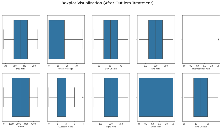
We limit the scope (even we know the outliers are still existed in two features). But, if we compare to our previous result, the latest version is much better even we can said it’s far away from perfectness. And it can be assumed that the final result can be used for further analysis (as modeling material in the next phase).

4. Visualize The Distributions

figure, ax = plt.subplots(2,5, figsize=(20,10))

#See the distribution of the data

plt.suptitle('Distribution of 10 Selected Features', size = 20)
sns.distplot(X['Day_Mins'],ax=ax[0,0])
sns.distplot(X['VMail_Message'], ax=ax[0,1])
sns.distplot(X['Day_Charge'], ax=ax[0,2])
sns.distplot(X['Eve_Mins'], ax=ax[0,3])
sns.distplot(X['International_Plan'], ax=ax[0,4])
sns.distplot(X['Phone'], ax=ax[1,0])
sns.distplot(X['CustServ_Calls'], ax=ax[1,1])
sns.distplot(X['Night_Mins'], ax=ax[1,2])
sns.distplot(X['VMail_Plan'], ax=ax[1,3])
sns.distplot(X['Eve_Charge'], ax=ax[1,4])
#plt.savefig('[Fig 3.2] Distribution of 10 Selected Features.png', dpi = 300)
plt.show()

png

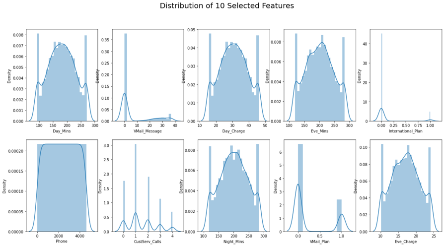
The distribution looks fine, go for further analysis.

5. Perform Heatmap Visualization

tri = X.copy()
tri['Churn'] = y
tri.head()

	Day_Mins	VMail_Message	Day_Charge	Eve_Mins	International_Plan	Phone	CustServ_Calls	Night_Mins	VMail_Plan	Eve_Charge
1	265.1	25	45.07	197.40	0	2637	1	244.7	1	16.780
2	161.6	26	27.47	195.50	0	2132	1	254.4	1	16.620
3	243.4	0	41.38	121.20	0	1509	0	162.6	0	10.300
4	271.1	0	46.09	118.78	1	2326	2	196.9	0	10.098
5	166.7	0	28.34	148.30	1	150	3	186.9	0	12.610

#Heatmap to shows the correlation

plt.figure(figsize=(20,15))
sns.heatmap(tri.corr(),cmap='nipy_spectral',annot=True)
plt.title('Heatmap of 10 Selected Features + Target',
         fontsize=25)
#plt.savefig('[Fig 3.3] Heatmap of 10 Selected Features and Target.png', dpi = 300)
plt.show()

png

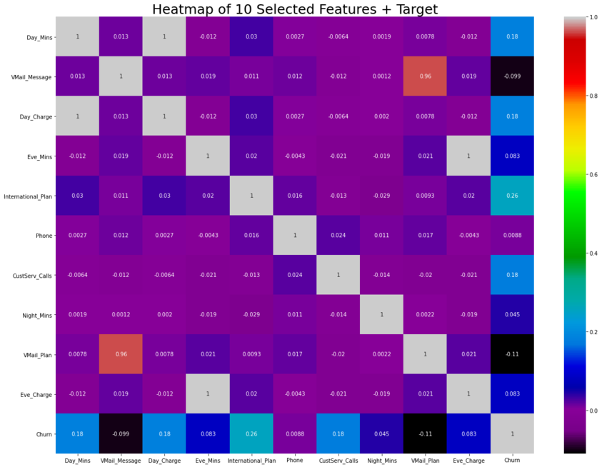
According to heatmap result, the most correlated features (indicated by the highest value) are: Eve_Mins >< Eve_Charge, VMail_Message >< VMail_Plan, Day_Charge >< Day_Mins. We will involve them for further demystification, and consider it as an alternative if our modeling is not working well..

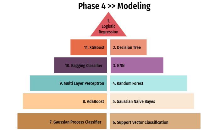png We vigorously believe when it comes to ML algorithm, "One Size Doesn't Fit All". The same things additionally occur when it comes to prediction. To resolve the issue, several classification models will be utilized for the comparative analysis and the best model (shown by accuracy score) will be chosen for this project. These are the list of our models for classification problem:

Logistic Regression
Decision Tree
KNN
Random Forest
Gaussian NB
SVC
Gaussian Process Classifier
AdaBoost
Multi Layer Perceptron (MLP)
Bagging Classifier
XGBoost Modeling

y.value_counts()

0    3961
1     656
Name: Churn, dtype: int64

As we can see above, the result 0 is majority (85%) and the rest of it is represent by 1 (15%). If we continue the modeling phase using this data, it will indicates misclassification.
Decision: treat imbalanced data using SMOTE.

# As the data is imbalanced we are using SMOTE to make sure that the value counts for the binary classes is the same

# imbalanced datasets will give imparied prediction results as the model is trained with higher emphasis on one class versus the other

from imblearn.over_sampling import SMOTE   #importing smote
oversampling =  SMOTE() #initializing SMOTE
x_smote, y_smote  = oversampling.fit_resample(X.astype('float'), y)
print(x_smote.shape, y_smote.shape)

(7922, 10) (7922,)

# checking to see if the data set is balanced

a = pd.DataFrame(y_smote)
print(a.value_counts())

Churn
0        3961
1        3961
dtype: int64

Now our data is balanced.
Decision: move forward to scaling the features.

##feature scaling > Reason being, the feature scaling was implemented to prevent any skewness in the contour plot of
#the cost function which affects the gradient descent but the analytical solution using normal equation does not suffer from the
#same drawback.

from sklearn.preprocessing import StandardScaler
sc = StandardScaler()

x_scaled =  sc.fit_transform(x_smote)
X_sc = pd.DataFrame(x_scaled)

# checking X 

X_sc.columns = list(X.columns)
X_sc.head()

	Day_Mins	VMail_Message	Day_Charge	Eve_Mins	International_Plan	Phone	CustServ_Calls	Night_Mins	VMail_Plan	Eve_Charge
0	1.395420	1.599364	1.395620	-0.160002	-0.497413	0.240178	-0.603658	0.974279	2.000813	-0.159833
1	-0.532285	1.684772	-0.532578	-0.202718	-0.497413	-0.141030	-0.603658	1.195312	2.000813	-0.202152
2	0.991254	-0.535830	0.991356	-1.873142	-0.497413	-0.611312	-1.401237	-0.896520	-0.550401	-1.873761
3	1.507171	-0.535830	1.507368	-1.927549	2.448922	0.005414	0.193921	-0.114932	-0.550401	-1.927189
4	-0.437296	-0.535830	-0.437264	-1.263876	2.448922	-1.637176	0.991499	-0.342800	-0.550401	-1.262777

def churn_predict(algorithm, training_x, testing_x, training_y, testing_y, cf, threshold_plot):
    #modeling
    algorithm.fit(training_x, training_y)
    predictions = algorithm.predict(testing_x)
    probabilities = algorithm.predict_proba(testing_x)
        
    print('Algorithm:', type(algorithm).__name__)
    print("\nClassification report:\n", classification_report(testing_y, predictions))
    print("Accuracy Score:", accuracy_score(testing_y, predictions))
    
    #confusion matrix
    conf_matrix = confusion_matrix(testing_y, predictions)

X_train, X_test, y_train, y_test = train_test_split(X_sc, y_smote, test_size=0.33, random_state=42, stratify=y_smote) #stratify -> it can reduce the variability of sample statistics
X_train.shape, X_test.shape, y_train.shape, y_test.shape

((5307, 10), (2615, 10), (5307,), (2615,))

1. Logistic Regression

from sklearn.linear_model import LogisticRegression

#Baseline model        
logit = LogisticRegression()

logit_acc = churn_predict(logit, X_train, X_test, y_train, y_test, "coefficients", threshold_plot=True)
logit_acc

Algorithm: LogisticRegression

Classification report:
               precision    recall  f1-score   support

           0       0.79      0.77      0.78      1308
           1       0.77      0.80      0.78      1307

    accuracy                           0.78      2615
   macro avg       0.78      0.78      0.78      2615
weighted avg       0.78      0.78      0.78      2615

Accuracy Score: 0.7808795411089866

Looks nice, but not good enough. So let’s doing a little improvement by comparing threshold, expecting better accuracies than above.

def predict_threshold (model,X_test,thresholds):
    return np.where(logit.predict_proba(X_test)[:,1]>thresholds,1,0)

for thr in np.arange(0,1.1,0.1):
    y_predict = predict_threshold(logit,X_test,thr)
    print("Threshold :",thr)
    print(confusion_matrix(y_test,y_predict))
    print("accuracy score for threshold" , thr , "is", accuracy_score(y_test, y_predict))

Threshold : 0.0
[[   0 1308]
 [   0 1307]]
accuracy score for threshold 0.0 is 0.49980879541108986
Threshold : 0.1
[[ 199 1109]
 [   6 1301]]
accuracy score for threshold 0.1 is 0.5736137667304015
Threshold : 0.2
[[ 452  856]
 [  48 1259]]
accuracy score for threshold 0.2 is 0.654302103250478
Threshold : 0.30000000000000004
[[ 698  610]
 [  87 1220]]
accuracy score for threshold 0.30000000000000004 is 0.7334608030592734
Threshold : 0.4
[[ 867  441]
 [ 150 1157]]
accuracy score for threshold 0.4 is 0.7739961759082218
Threshold : 0.5
[[1002  306]
 [ 267 1040]]
accuracy score for threshold 0.5 is 0.7808795411089866
Threshold : 0.6000000000000001
[[1094  214]
 [ 455  852]]
accuracy score for threshold 0.6000000000000001 is 0.7441682600382409
Threshold : 0.7000000000000001
[[1159  149]
 [ 705  602]]
accuracy score for threshold 0.7000000000000001 is 0.6734225621414914
Threshold : 0.8
[[1217   91]
 [ 927  380]]
accuracy score for threshold 0.8 is 0.6107074569789674
Threshold : 0.9
[[1271   37]
 [1121  186]]
accuracy score for threshold 0.9 is 0.55717017208413
Threshold : 1.0
[[1308    0]
 [1307    0]]
accuracy score for threshold 1.0 is 0.5001912045889101

It is evident from the above that the optimal threshold is 0.5 which is the default threshold.
Accuracy score is low as expected as the data is quite complex with no clear distinct boundaries for the two classes. Logistic regression models cannot be used for such complex data sets.

#Hyperparameter Tuning
from sklearn.model_selection import GridSearchCV

from sklearn.tree import DecisionTreeClassifier
from sklearn import tree

2. Decision Tree

# Model building - hyperparam tuning


Deci_Tree_model  = DecisionTreeClassifier()

parameters = {'max_depth':[3,5,7,9,10],
              'random_state': [10,50,100,123,154],
              'splitter':['best', 'random'],
              'criterion':['gini', 'entropy']
             }  

grid = GridSearchCV(Deci_Tree_model,parameters,cv=5,verbose=1) 
grid.fit(X_train,y_train)

print('Best parameter of Decision Tree Algorithm:\n',grid.best_params_)

Fitting 5 folds for each of 100 candidates, totalling 500 fits
Best parameter of Decision Tree Algorithm:
 {'criterion': 'entropy', 'max_depth': 9, 'random_state': 100, 'splitter': 'best'}

Deci_Tree_model = DecisionTreeClassifier(criterion = 'entropy', max_depth = 9, 
                                         random_state = 100, splitter = 'best')
Deci_Tree_model_acc = churn_predict(Deci_Tree_model, X_train, X_test, y_train, y_test, "features", threshold_plot=True)
Deci_Tree_model_acc

Algorithm: DecisionTreeClassifier

Classification report:
               precision    recall  f1-score   support

           0       0.94      0.93      0.94      1308
           1       0.93      0.94      0.94      1307

    accuracy                           0.94      2615
   macro avg       0.94      0.94      0.94      2615
weighted avg       0.94      0.94      0.94      2615

Accuracy Score: 0.9365200764818356

3. KNN

# Model building - hyperparam tuning

from sklearn.neighbors import KNeighborsClassifier
knn  = KNeighborsClassifier()

parameters = {'n_neighbors':[5,10,20,50,75],
              'weights': ['uniform','distance'],
              'algorithm':['auto', 'ball_tree', 'kd_tree', 'brute'],
              'leaf_size':[5, 7, 10, 20, 30],
             }  

grid = GridSearchCV(knn,parameters,cv=5,verbose=1) 
grid.fit(X_train,y_train)

print('Best parameter of KNeighborsClassifier Algorithm:\n',grid.best_params_)

Fitting 5 folds for each of 200 candidates, totalling 1000 fits
Best parameter of KNeighborsClassifier Algorithm:
{'algorithm': 'auto', 'leaf_size': 5, 'n_neighbors': 5, 'weights': 'distance'}

knn = KNeighborsClassifier(algorithm='auto', leaf_size=5, 
                           n_neighbors=5, p=2, weights='distance')
knn_acc = churn_predict(knn, X_train, X_test, y_train, y_test, 'None', threshold_plot=True)
knn_acc

Algorithm: KNeighborsClassifier

Classification report:
               precision    recall  f1-score   support

           0       0.95      0.85      0.90      1308
           1       0.87      0.95      0.91      1307

    accuracy                           0.90      2615
   macro avg       0.91      0.90      0.90      2615
weighted avg       0.91      0.90      0.90      2615

Accuracy Score: 0.9032504780114723

4. Random Forest

# Model building - hyperparam tuning

from sklearn.ensemble import RandomForestClassifier
rfc  = RandomForestClassifier()

parameters = {'n_estimators':[10,25,50,100],
              'random_state': [20, 50, 74, 123],
              'max_depth':[3, 5, 9, 10],
              'criterion':['gini', 'entropy'],
             }  

grid = GridSearchCV(rfc,parameters,cv=5,verbose=1) 
grid.fit(X_train,y_train)

print('Best parameter of RandomForestClassifier Algorithm:\n',grid.best_params_)

Fitting 5 folds for each of 128 candidates, totalling 640 fits
Best parameter of RandomForestClassifier Algorithm:
 {'criterion': 'entropy', 'max_depth': 10, 'n_estimators': 50, 'random_state': 20}

rfc = RandomForestClassifier(n_estimators = 50, random_state = 20,
                             max_depth = 10, criterion = "entropy")

rfc_acc = churn_predict(rfc, X_train, X_test, y_train, y_test, 'features', threshold_plot=True)
rfc_acc

Algorithm: RandomForestClassifier

Classification report:
               precision    recall  f1-score   support

           0       0.92      0.93      0.92      1308
           1       0.93      0.91      0.92      1307

    accuracy                           0.92      2615
   macro avg       0.92      0.92      0.92      2615
weighted avg       0.92      0.92      0.92      2615

Accuracy Score: 0.9223709369024856

5. Gaussian NB

from sklearn.naive_bayes import GaussianNB

gnb = GaussianNB(priors=None)

gnb_acc = churn_predict(gnb, X_train, X_test, y_train, y_test, 'None', threshold_plot=True)
gnb_acc

Algorithm: GaussianNB

Classification report:
               precision    recall  f1-score   support

           0       0.79      0.71      0.75      1308
           1       0.74      0.81      0.77      1307

    accuracy                           0.76      2615
   macro avg       0.76      0.76      0.76      2615
weighted avg       0.76      0.76      0.76      2615

Accuracy Score: 0.7621414913957935

6. SVC

# Model building - hyperparam tuning

from sklearn.svm import SVC
svc  = SVC()

parameters = {'C':[0, 1, 7.8, 10],
              'kernel': ['rbf', 'sigmoid'],
              'gamma':['scale', 'auto'],
              'random_state':[10, 59, 74, 124],
             }  

grid = GridSearchCV(svc,parameters,cv=5,verbose=1) 
grid.fit(X_train,y_train)

print('Best parameter of SVC Algorithm:\n',grid.best_params_)

Fitting 5 folds for each of 64 candidates, totalling 320 fits
Best parameter of SVC Algorithm:
 {'C': 10, 'gamma': 'auto', 'kernel': 'rbf', 'random_state': 10}

svc  = SVC(C=10, kernel='rbf', gamma='auto', probability=True, random_state=10)

svc_acc = churn_predict(svc, X_train, X_test, y_train, y_test, "coefficients", threshold_plot=True)
svc_acc

Algorithm: SVC

Classification report:
               precision    recall  f1-score   support

           0       0.91      0.93      0.92      1308
           1       0.93      0.91      0.92      1307

    accuracy                           0.92      2615
   macro avg       0.92      0.92      0.92      2615
weighted avg       0.92      0.92      0.92      2615

Accuracy Score: 0.9193116634799235

7. Gaussian Process Classifier

from sklearn.gaussian_process import GaussianProcessClassifier

gpc = GaussianProcessClassifier(random_state=124)

gpc_acc = churn_predict(gpc, X_train, X_test, y_train, y_test, "None", threshold_plot=True)
gpc_acc

Algorithm: GaussianProcessClassifier

Classification report:
               precision    recall  f1-score   support

           0       0.91      0.89      0.90      1308
           1       0.90      0.91      0.90      1307

    accuracy                           0.90      2615
   macro avg       0.90      0.90      0.90      2615
weighted avg       0.90      0.90      0.90      2615

Accuracy Score: 0.9021032504780114

8. AdaBoost

from sklearn.ensemble import AdaBoostClassifier
# Model building - hyperparam tuning

adac  = AdaBoostClassifier()

parameters = {'algorithm':['SAMME', 'SAMME.R'],
              'n_estimators': [5, 10, 25, 50],
              'learning_rate':[0.5, 0.8, 1.0, 2.5],
              'random_state':[10, 59, 74, 124],
             }  

grid = GridSearchCV(adac,parameters,cv=5,verbose=1) 
grid.fit(X_train,y_train)

print('Best parameter of AdaBoostClassifier Algorithm:\n',grid.best_params_)

Fitting 5 folds for each of 128 candidates, totalling 640 fits
Best parameter of AdaBoostClassifier Algorithm:
 {'algorithm': 'SAMME.R', 'learning_rate': 1.0, 'n_estimators': 50, 'random_state': 10}

adac = AdaBoostClassifier(algorithm = 'SAMME.R', learning_rate = 1.0,n_estimators = 50, random_state=10)

adac_acc = churn_predict(adac, X_train, X_test, y_train, y_test, "features", threshold_plot=True)
adac_acc

Algorithm: AdaBoostClassifier

Classification report:
               precision    recall  f1-score   support

           0       0.91      0.91      0.91      1308
           1       0.91      0.91      0.91      1307

    accuracy                           0.91      2615
   macro avg       0.91      0.91      0.91      2615
weighted avg       0.91      0.91      0.91      2615

Accuracy Score: 0.9105162523900574

9. Multi Layer Perceptron

from sklearn.neural_network import MLPClassifier

mlp = MLPClassifier()

parameters = {'solver':['lbfgs', 'sgd', 'adam'],
              'activation': ['tanh', 'relu'],
              'alpha':[1, 10],
              'max_iter':[50, 100],
              'random_state':[5, 50, 124],
             }  

grid = GridSearchCV(mlp,parameters,cv=5,verbose=1) 
grid.fit(X_train,y_train)

print('Best parameter of MLPClassifier Algorithm:\n',grid.best_params_)

Fitting 5 folds for each of 72 candidates, totalling 360 fits
Best parameter of MLPClassifier Algorithm:
 {'activation': 'relu', 'alpha': 1, 'max_iter': 100, 'random_state': 124, 'solver': 'lbfgs'}

mlp = MLPClassifier(activation = 'relu', alpha = 1, 
                    max_iter = 100, random_state = 124, 
                    solver = 'lbfgs')

mlp_acc = churn_predict(mlp, X_train, X_test, y_train, y_test, "None", threshold_plot=True)
mlp_acc

Algorithm: MLPClassifier

Classification report:
               precision    recall  f1-score   support

           0       0.92      0.92      0.92      1308
           1       0.92      0.91      0.92      1307

    accuracy                           0.92      2615
   macro avg       0.92      0.92      0.92      2615
weighted avg       0.92      0.92      0.92      2615

Accuracy Score: 0.918546845124283

10. Bagging Classifier

# >< no need hyperparameter tuning

from sklearn.ensemble import BaggingClassifier

bgc = BaggingClassifier(random_state=124)

bgc_acc = churn_predict(bgc, X_train, X_test, y_train, y_test, "None", threshold_plot=True)
bgc_acc

Algorithm: BaggingClassifier

Classification report:
               precision    recall  f1-score   support

           0       0.93      0.95      0.94      1308
           1       0.95      0.93      0.94      1307

    accuracy                           0.94      2615
   macro avg       0.94      0.94      0.94      2615
weighted avg       0.94      0.94      0.94      2615

Accuracy Score: 0.9384321223709369

11. XGBoost

from xgboost import XGBClassifier

xgb = XGBClassifier()

estimator = XGBClassifier(
    objective= 'binary:logistic',
    nthread=4,
    seed=42
)

parameters = {'max_depth': range (2, 10, 1),
              'n_estimators': range(60, 220, 40),
              'learning_rate': [0.1, 0.01, 0.05]
             }  

grid = GridSearchCV(estimator=estimator,param_grid=parameters,scoring = 'accuracy',n_jobs = 10,cv = 10,verbose=True) 
grid.fit(X_train,y_train)

print('Best parameter of XGBClassifier Algorithm:\n',grid.best_params_)

Fitting 10 folds for each of 96 candidates, totalling 960 fits
[08:16:58] WARNING: C:/Users/Administrator/workspace/xgboost-win64_release_1.4.0/src/learner.cc:1095: Starting in XGBoost 1.3.0, the default evaluation metric used with the objective 'binary:logistic' was changed from 'error' to 'logloss'. Explicitly set eval_metric if you'd like to restore the old behavior.
Best parameter of XGBClassifier Algorithm:
 {'learning_rate': 0.1, 'max_depth': 9, 'n_estimators': 180}

xgb = XGBClassifier(learning_rate = 0.1, max_depth=9, n_estimators = 180)

xgb_acc = churn_predict(xgb, X_train, X_test, y_train, y_test, "None", threshold_plot=True)
xgb_acc

[08:20:36] WARNING: C:/Users/Administrator/workspace/xgboost-win64_release_1.4.0/src/learner.cc:1095: Starting in XGBoost 1.3.0, the default evaluation metric used with the objective 'binary:logistic' was changed from 'error' to 'logloss'. Explicitly set eval_metric if you'd like to restore the old behavior.
Algorithm: XGBClassifier

Classification report:
               precision    recall  f1-score   support

           0       0.96      0.95      0.96      1308
           1       0.95      0.96      0.96      1307

    accuracy                           0.96      2615
   macro avg       0.96      0.96      0.96      2615
weighted avg       0.96      0.96      0.96      2615

Accuracy Score: 0.955640535372849

png -) Summary of the Analysis

#wrap up each accuracies into variables
xgb_ac = 0.955640535372849
bgc_ac = 0.9384321223709369
mlp_acc = 0.918546845124283
adac_acc = 0.9105162523900574
gpc_acc = 0.9021032504780114
svc_acc = 0.9193116634799235
gnb_acc = 0.7621414913957935
rfc_acc = 0.9223709369024856
knn_acc = 0.9032504780114723
Deci_Tree_model_acc = 0.9365200764818356
logit_acc = 0.7808795411089866

# Summary of the Accuracy scores for test data
model_ev = pd.DataFrame({'Model': ['Logistic Regression','Decision Tree','KNN','Random Forest',
                    'Gaussian NB','SVC', 'Gaussian Process', 'AdaBoost', 'MLP', 'Bagging', 'XGBoost'],
                         'Accuracy_percentage': [round(logit_acc*100, 2), round(Deci_Tree_model_acc*100, 2),round(knn_acc*100, 2),
                                          round(rfc_acc*100, 2),round(gnb_acc*100, 2),round(svc_acc*100, 2),
                                          round(gpc_acc*100, 2), round(adac_acc*100, 2), round(mlp_acc*100, 2),
                                          round(bgc_ac*100, 2), round(xgb_ac*100, 2)]})
table_train = ff.create_table(model_ev)
py.iplot(table_train)

png

# Use textposition='auto' for direct text
fig = go.Figure(data=[go.Bar(
            x=model_ev.Model, y=model_ev.Accuracy_percentage,
            text=model_ev.Accuracy_percentage,
            textposition='auto',
        )])

fig.show()

png

This visualization is better, concise, and easy to understand than seeing the accuracy results one by one in phase 4.

We’ve prosperously reached the entire project goal as represented in the details above on each phase, and here are the conclusions:

10 selected features could be able to influence the “churn rate”. And it would be able to affect the customer behavior.
By trying various models, we could compare each accuracy so the predicted churn risk score (which is represented by Y) is much more sensible to drive retention campaigns and the email campaigns (which contain lucrative offers) could be successfully hitting the target to Churn-YES customers.

-) Recommendations:

Eventually we knew that most of our models are felicitous (denoted by the percentage of accuracy > 90%), we highly recommend to applied XGBoost model for this client project because it shows higher accuracy.
Build the algorithm to provide a chatbot feature (virtual assistant that could possibly avail the customer to solve their issues) and locate it inside downloadable apps and official website. With the help of chatbot existence, it comes in handy when it comes to auto categorizing tickets, request fulfillment, customer care support, and any other issues.
Collaborating with IT field to discuss more the algorithm, including the UI & UX design (which is liable to affect customer satisfaction and this can lead to churn-flag-yes). So the customers could leave reviews after using the chatbot features. And we can use their reviews as a further evaluation and analysis.

-) Project Risks:

This dataset contains pretty much outliers, so the most consuming time to do the analysis is by comparing different methods of outlier treatments. We have to try them one by one and visually perceive which method is suitable to solve them well and ascertain no mistakes while doing them.
Some of the models while doing hyperparameter tuning, it took a long time to execute. We can understand it because every PC specification is different. Consequently, some of us use GoogleColab as an alternative solution.

← Previous Post